Graphs in Machine Learning applications

What have we learned from Graph-Powered Machine Learning so far?

• What machine learning is
• What graphs are
• Machine learning and graphs are a perfect fit
• What big data is and that big data and machine learning are almost inseparable
• Big data and graphs are an ideal fit

Now, in the book’s third chapter, the author Alessandro Negro ties all this together. The chapter focuses on Graphs in machine learning applications. Following the machine learning project life cycle, we’ll go through: managing data sources, algorithms, storing and accessing data models, and visualisation.

You will first learn how to transform raw data into a graph from this article. Then, we’ll go through some of the graph data science algorithms and their uses. And finally, we’ll touch upon the importance of storing and visualising ML models.

From raw data to graph - managing data sources

Creating a single connected source of truth - a graph connecting all your data - helps you manage and prepare your data. This graph can be created by graph modelling and graph construction. In graph modelling, the graph is a different, connected, representation of the existing data. In graph construction the graph is created by relating data points that in their original sources appeared as unrelated. Applying an edge construction mechanism builds connections, and thus enriches the original dataset with a brand new set of information.

When creating a graph from your data you need to:

1. Identify data sources. Identify the data you have as well as external data sources that can enrich your data.
2. Analyse the data available. Machine learning projects need large quantities of high-quality training data. Thus it is important to evaluate the quality of all your data sources.
3. Design the graph data model. Here you ought to decide which data you need to extract from the data sources, and create a graph model for this data.
4. Define the data flow. Design a flow extracting, transforming, and loading (ETL) data into the graph.
5. Import data into the graph.
6. Perform post-import tasks:
   1. Data cleaning - tackle incomplete or incorrect data.
   2. Data enrichment - enrich your data with external data sources.
   3. Data merging - merge duplicates and connect related items.

Algorithms

Once your data is in a graph, it’s time to perform the initial analysis with graph data science algorithms. The following is not an exhaustive list; however, it will provide you with a basic understanding of what graph algorithms can do.

Centrality algorithms

Centrality algorithms help identify the most important nodes in a network. This is useful e.g., in communication/social networks or supply chains: they allow you to identify “bridges” in a social network, single point of failure in a communication network, key providers in a supply chain. Centrality algorithms are also helpful when performing risk analyses.

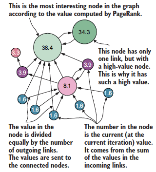
Page Rank algorithm assesses the importance of a node by the number of relationships to and from it and the relevance of the nodes connected to it. The more relationships, the more important the node is. The higher valued nodes connect to a node, the higher its score.

One application of PageRank is assessing the quality of scientific articles. If many articles cite one specific article, that article is likely to be a quality piece of work. The higher the quality of the articles linking to it, the better.

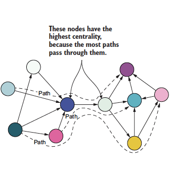
Betweenness centrality algorithms count the number of shortest paths a node is on. High centrality nodes lie on many shortest paths.

Betweenness centrality can detect the key nodes in a network. In communication networks, the key nodes help you quickly get a message to the whole network. The key nodes need to be protected in the supply chain, as their failure would affect a large part of the supply chain.

Keyword extraction and co-occurrence

Graph databases can store unstructured data (free text). To group, organise, index, process, and get insights from this data, you need to first extract keywords from it. This is an example of graph construction technique since it creates new nodes and new relationships not existing in the original data sources. You can extract keywords from documents in different ways:

Relative frequency criterion is the simplest method of keyword extraction. It identifies the most used words in a document. However, the most used words are not necessarily valuable keywords. Thus, this method yields sub-optimal results.

A more sophisticated (and accurate) method is supervised learning. Supervised learning uses machine learning to train a system to identify keywords. The downside of this method is the large amount of data needed to train the systems.

You can also use the TextRank (similar to PageRank) algorithm. You first look at the co-occurrence of words in a document to do so. If two words occur in the window of max N-words, they are connected by a relationship. TextRank then identifies keywords based on the number and strength of these connections using PageRank.

Graph clustering and community detection

Clustering algorithms identify clusters of densely connected nodes within a graph. The nodes in each cluster are only weakly connected to nodes in other clusters - making them distinct. Weakly Connected Components, Label Propagation, and Louvain are the most famous clustering algorithms. Read our blog about Graph Data Science at scale for an explanation of what these are and when to use them.

Collaborative filtering and item-based algorithms

These algorithms are especially useful when providing recommendations. Collaborative filtering leverages past user behaviour to make predictions about future behaviour/interests. An outcome is a numerical value indicating the likelihood of a said outcome - of a user liking a said item. An alternative are item based algorithms, which provide predictions based on item similarity.

Algorithms that aid with recommendations rely on similarity computations. In a typical implementation, the similarity is used to find items similar to the items a user liked or purchased already. Reducing the number of computations needed increases speed and improves performance. A bipartite graph representing user-item interaction reduces the number of computations needed to compute similarities among items or users. Bipartite graph (or bigraph) is a graph whose nodes can be divided into two independent sets. Each relationship connects a node from one set to a node in the other. Thus there are relationships between the two sets, but no relationships within them. In such a graph, you can use a simple query to find overlapping items – i.e. items sharing one or more interested users. Excluding all the non-overlapping items (since they will have similarity of 0), considerably reduces the number of computations needed for a recommendation, thus speeding up the process. Alternatively, you can separate bipartite graphs into clusters. Then you only need to compute similarities among the items within the same cluster.

Storing and accessing machine learning models

Once you’ve applied the algorithms, machine learning models are ready to provide recommendations. To do this, the machine learning models need to be stored somewhere. The way the models are stored impacts the speed and ease of their access. The speed of access patterns affects the speed of the end recommendations. Thus, how you store machine learning models affects their performance.

As I discussed in the last blog, graphs provide fast access patterns. Graphs are also indexed by both relationships and nodes - further speeding up data access. Hence, graphs are ideal for storing machine learning models, such as similarities, factorizations, and similar.

Visualisation

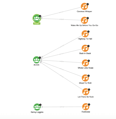
Data visualisations help us make sense of connected data. They help us understand, as well as analyse, the data further. Leveraging our (human) pattern-recognition abilities, it’s easy to understand and interpret visualised data. Graph visualisations make it easier to spot patterns, outliers, and gaps.

Conclusion

To sum it up, graphs are an ideal companion for your machine learning project. With graphs, you can:

• create a single source of truth,
• leverage graph data science algorithms,
• store and access ML models quickly, and
• visualise the models and their outcomes.

Are you ready to start your graph journey? Get in touch with our experts and leverage the power of graphs, graph-data science algorithms, and graph-powered insights.