Only a few things are more satisfying for a graph data scientist than playing with Neo4j Graph Data Science library algorithms, most probably running them in production and at scale. Possibly also using them to fight against scammers and fraudsters who threaten your business.
A key element in fighting scams and fraud is the Account Association. It is crucial to know if an account belongs to a legitimate user or is part of a set of accounts used by malicious users to circumvent your anti-fraud and anti-scam measures.
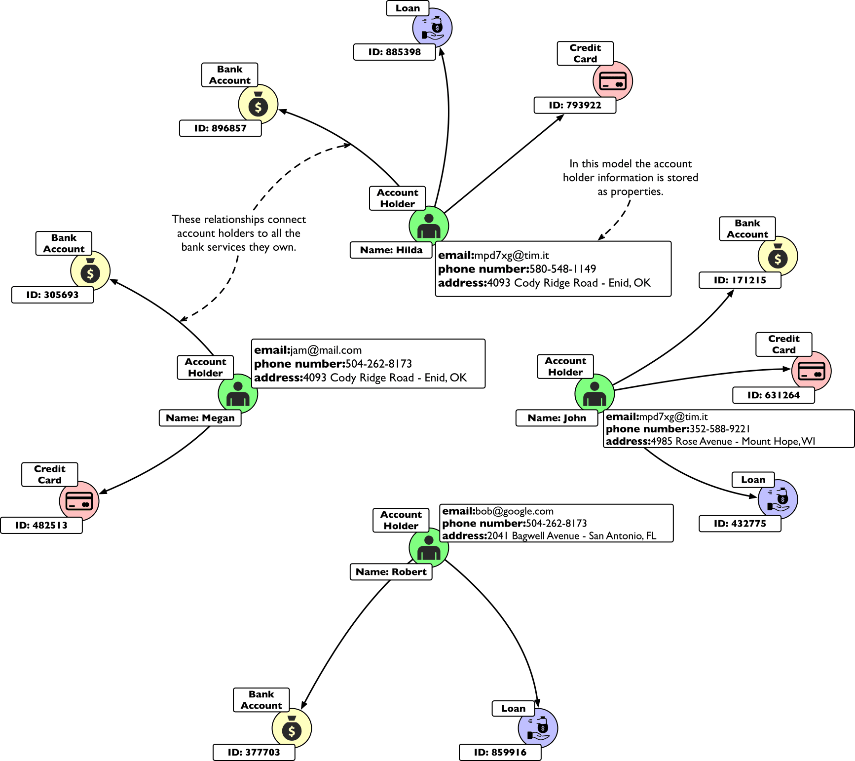
This image shows how a few, apparently unrelated, bank account holders actually share some properties. This can be even more explicit if we materialise the properties as nodes and we connect accounts through them:
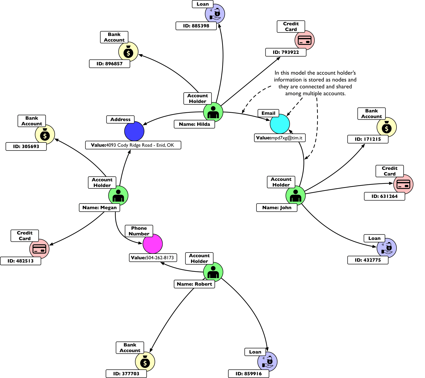
In this example, Robert is directly connected to Megan but also indirectly connected to Hilda and John.
Fraudsters and scammers will actively try to hide these kinds of relationships by faking email addresses and phone numbers or altering the shipping address slightly.
On the other hand, the more properties are available to connect people, the lower the chances that they will manage to alter or hide them all.
Moreover, graphs make it easy to spot indirect connections. This leaves an even smaller hiding surface for adversaries, especially when they try to scale their activities.
Clustering
GDS gives us different options for clustering accounts that share some direct or indirect connections. All these algorithms fall under the Community Detection category. Let’s explore some of them.
WCC
The simplest community detection algorithm is the Weakly Connected Component. It is very easy and fast, and can be used to generate subgraphs of accounts. Its primary drawback is that it assumes all connections to be true, so extra care is needed if there is a chance for false-positive shared properties.
Label propagation algorithm
A fast alternative to WCC, which is more tolerant of false positives, is the Label Propagation Algorithm (LPA). LPA uses an iterative approach to form clusters if there is some supporting evidence from the surroundings. This mimics the way domain experts decide about false-positive associated accounts.
Louvain
The last item in our brief overview is the Louvain algorithm. The algorithm compares the connectivity of a candidate community against the connectivity of a random network. This comparison is used to estimate the quality of the assignment of nodes to a potential community.
Louvain uses a hierarchical approach, iteratively condensing communities into nodes, making this algorithm very suitable for handling large networks.
We can generalise the Account Association solution as a two-step task: model your graph to capture connected facts (like shared properties) and run a community detection algorithm to generate clusters of connected accounts.
Infrastructure
It is not uncommon to have millions of users connected through potentially billions of shared properties or facts. If this is your case, you definitely should design a system that gives you both performance and reliability.
Neo4j provides a big help in this sense with Neo4j’s Causal Cluster.
Under the Causal Cluster architecture, each node can play the role of Primary server or Secondary server.
Primary server
Primary servers are the core instances
They are collectively responsible for data safety, which means that only the simple majority of core nodes are required to acknowledge a transaction so the cluster can tolerate faults.
Secondary server
Secondary servers are defined as Read Replica instances. They are asynchronously replicated from Primary Servers via transaction log shipping.
The primary purpose of the Read Replica instances is to scale out read workloads, but they also serve as a lifesaver in case of disaster recovery.
Causal consistency
The causal consistency is one possible consistency model used in distributed computing. It ensures that clients can read at least their own writing, regardless of which instance they communicate with. This simplifies the client’s logic, which can treat a large cluster as if it were a single (logical) server.
Here is an extremely condensed picture of how a read replica works together with a core node to increase read throughput.
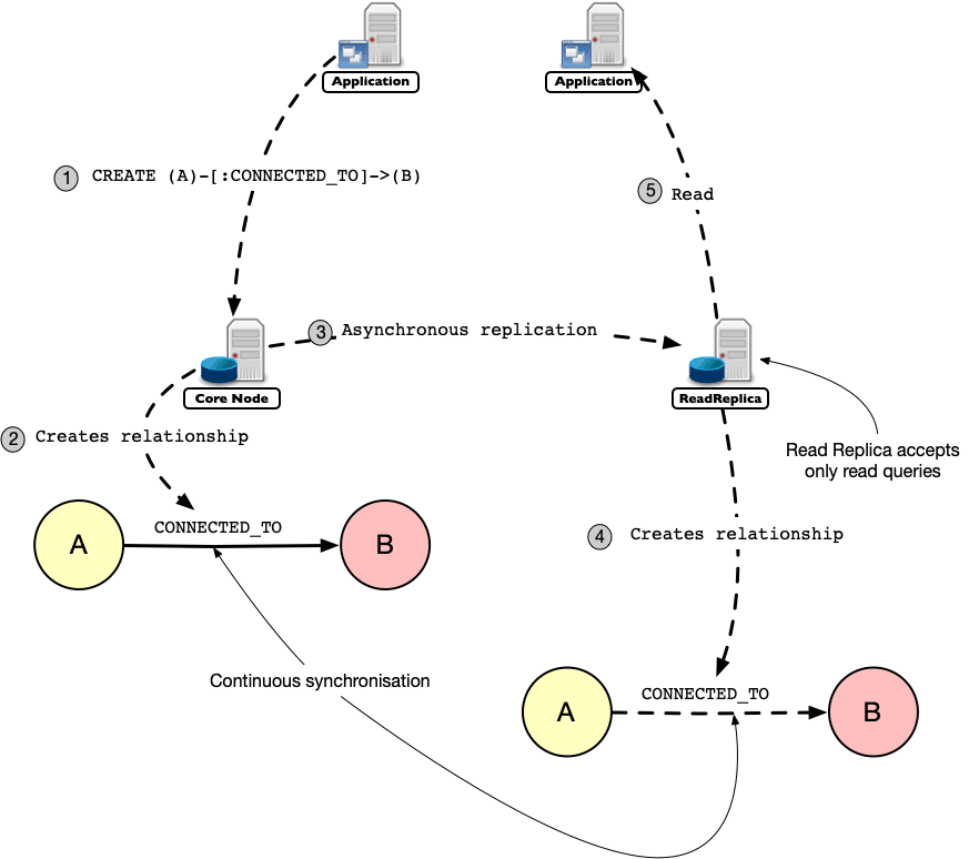
With a three-node configuration spread in three different datacenters, we can provide a robust environment in which you can easily ingest and process daily updates from your operational data sources.
GDS & causal clusters
Once the architecture has been designed and servers have been configured, we can come back to our original goal: fighting fraudsters and scammers.
The only thing left is installing GDS and starting our Account Association journey, seeking scammers and fraudsters.
While it may sound reasonable to just install GDS on the core cluster, as we were in a single-node deployment, we must be aware of the drawbacks.
GDS workloads can be very memory hungry, and algorithms can hold the CPUs long enough to interfere with the heartbeat mechanism of the cluster protocol. This can make the node appear as if it were faulty to the rest of the cluster.
These are the main reasons why it is strongly discouraged to set up a GDS core node in a cluster.
On the other hand, running GDS workloads on a read replica ensures that data is always in sync, and computations will not interfere with the normal cluster operations.
This comes at a price. Read Replicas are read-only, and thus it is not possible to store back your algorithm’s results. If you don’t want to lose your freshly computed results, you have to store your data back to the cluster using some custom approach.
Here, GraphAware Hume comes to the rescue: by leveraging the ability of Hume’s Orchestra to handle different Neo4j resources at the same time, you can run a workflow that consumes results from the GDS-powered Read Replica and writes them back to the cluster in a breeze.
Let’s see how:
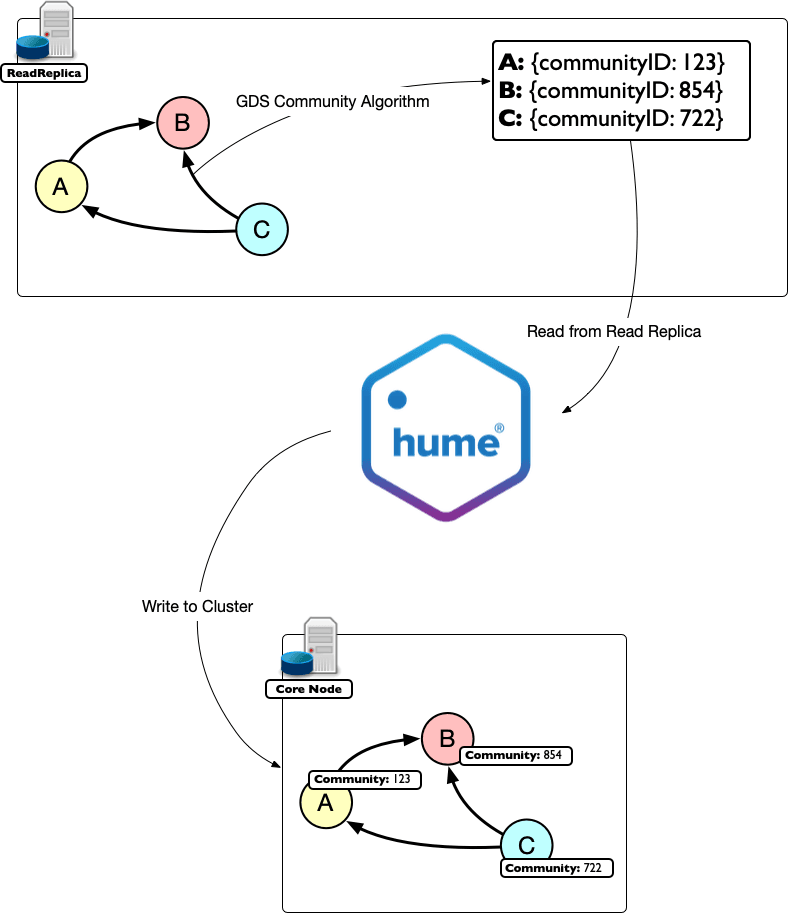
Here we use Hume’s Orchestra workflow to interact directly with the Read Replica server, asking it to compute a community detection algorithm.
We can not write the results back to the nodes in place since this would require the Read Replica node to generate a write transaction, and the Read Replica can only do reads.
We would rather configure the algorithm to run in a stream mode so that records can flow back into the Orchestra workflow. We then instruct the workflow to issue write queries to the core servers to update the relevant nodes according to the community algorithm results.
The Causal Consistency will do the rest: the newly created “Community” property will be available to the Read Replica node as well as to the rest of the cluster.
Practical example
As we saw, resolving Account Association means running a community detection algorithm over a graph model able to capture connecting facts. We also saw how GraphAware Hume can make it possible to decouple GDS algorithms in a Neo4j cluster setting.
Introducing the dataset
Let’s test these ideas with a concrete example. We will overcome the issue of finding a publicly available and properly sized scam/fraud-related dataset by using a movie-themed database instead.
Here is the knowledge graph schema based on the data available on the Internet Movie Database IMDb.

We will pretend that the Movie node is our “connecting fact” and the Person nodes are the accounts we are trying to associate.
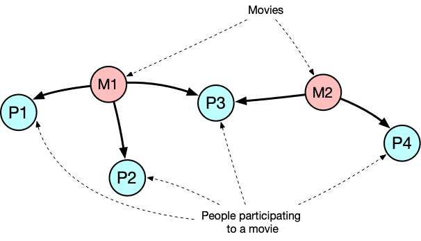
In this example, P1 is connected to P2 because they both participated in the movie M1, and P4 is connected to P3 because of the movie M2. Moreover, all these people are part of a connected component, so they can potentially belong to the same cluster.
Our Account Association problem becomes “finding communities of people connected by a common participation in some movie”. The community detection algorithm we choose will determine how those clusters will be shaped.
Prepare the data
Running a community detection algorithm in GDS is a two-step process. Graph algorithms, in fact, are designed to work with a graph data model, which is an in-memory projection of the Neo4j property graph data model. Projecting allows us to select only the relevant information and allows GDS to use in-memory, highly optimised data structures.
Therefore, the first step is to perform the projection, which means creating a named catalogue under the GDS architecture.
In GDS, we can create catalogues using either a Native or a Cypher projection.
The Cypher projection is the most flexible one, since we can write a query to project the nodes we want to store into the catalogue and another query to project the relationships connecting these nodes. We are completely free to apply any kind of transformations to both, so the graph in the catalogue can be potentially very different from the graph it comes from.
The Native projection is the simplest one. It can be as easy as selecting the label for nodes and relationships we are interested in. With native projection, we can also select more than one label or limit the properties we want to project, but we can not apply any transformation to the data. As you can imagine, native projections are far more performant compared to Cypher projections.
Due to the dimensionality of the graph (19.8M nodes, 135M relationships), we cannot compute a GDS catalogue straight from a Cypher query. We need to materialise a new relationship to connect two people if they both participate in the same movie.
Luckily, this is a very easy task to carry out using Hume Orchestra.
The idea is that we traverse all the movies in the database, and then we create a connection for every pair of people participating in that movie, if they are not already connected because of another movie we have already traversed.
We use a temporary node label to mark the movies yet to be visited, so the process can be interrupted and recovered if needed.
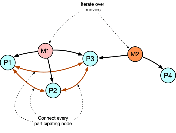
As soon as the process completes, we can create a catalogue in our GDS Read Replica node.
Creating the catalogue is as simple as running:
CALL gds.graph.create(
    "MoviesDB",
    "Person",
    "APPEARS_WITH")
Detect clusters
With the catalogue in place, we can finally run our community detection algorithm, but which one?
WCC is not suitable for this dataset; people participate in many movies, which can lead to a huge connected component that does not help us. In general, if your graph is densely connected, WCC makes sense only if you can preprocess relationships to keep only the relevant ones.
Label Propagation may also not be the perfect option here because of the size of the graph, and thus the number of iterations that could be required to let the algorithm converge.
Louvain looks very promising because of its hierarchical approach and its ability to distinguish random connections from real communities.
So let the magic happen with this workflow, seamlessly streaming Lovain results into our cluster:
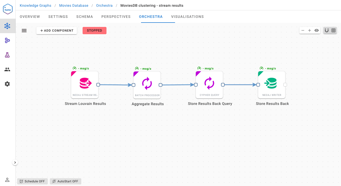
The first component executes the Louvain algorithm in stream mode over the catalogue we have just created. As soon as the results become available, it will start to send messages containing the nodeId with its associated clusterId.
The Batch Processor in the second position allows us to aggregate Louvain results so we can update multiple nodes in a single transaction.
The last two components perform the actual writing each time a batch is ready.
The ability to select different data sources at the component level allows us to easily transform and transfer data in a single workflow.
Explore the results
Once the workflow completes, our Person nodes get a new property representing their cluster ID.
Let’s create a visualisation and check the results of the process. Since we are going to only read data from the graph, let’s use a Read Replica node as the data source. We can enable the grouping function over the cluster ID to make the clusters visually clearer.
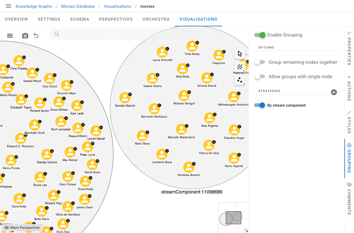
And here we are, Marcello Matroianni and Michelangelo Antonioni right next to Gary Cooper and Grace Kelly.
Louvain was able to separate actors and directors belonging to the classical and new Hollywood cinema from actors and directors belonging to the Italian golden age cinema. This kind of separation wouldn’t be possible by using WCC alone because there are many Hollywood actors and directors participating in Italian movies and vice versa, effectively leading to a single connected component.
More reliable approach
We saw how Hume made it possible to easily integrate GDS with Causal Clustering through Hume’s Orchestra and by leveraging the stream mode algorithm execution.
While streaming the Louvain outputs directly to the cluster is definitely easy and convenient, streaming may not be the safest way to move and store large amounts of data.
The GDS streaming execution, in fact, does not give you the chance to interrupt the process and recover it later if needed.
Here, we propose a slightly more articulated approach that is easier to track and tolerant to interruptions.
We combine the “mutate” mode and the “streamNodeProperties” function to actually “paginate” the algorithm’s results and thus also paginate the transfer to the cluster nodes.
Let’s see how in detail:
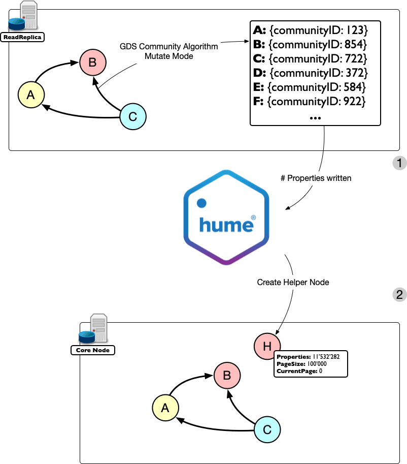
- We start by creating the catalogue and running the Louvain algorithm as usual, but this time we use the mutate mode. As a result, we get back the number of properties written to the in-memory graph.
- We note down the total number of mutated properties by writing it into a helper node, PagingHelper, which will allow us to keep track of the transfer process.
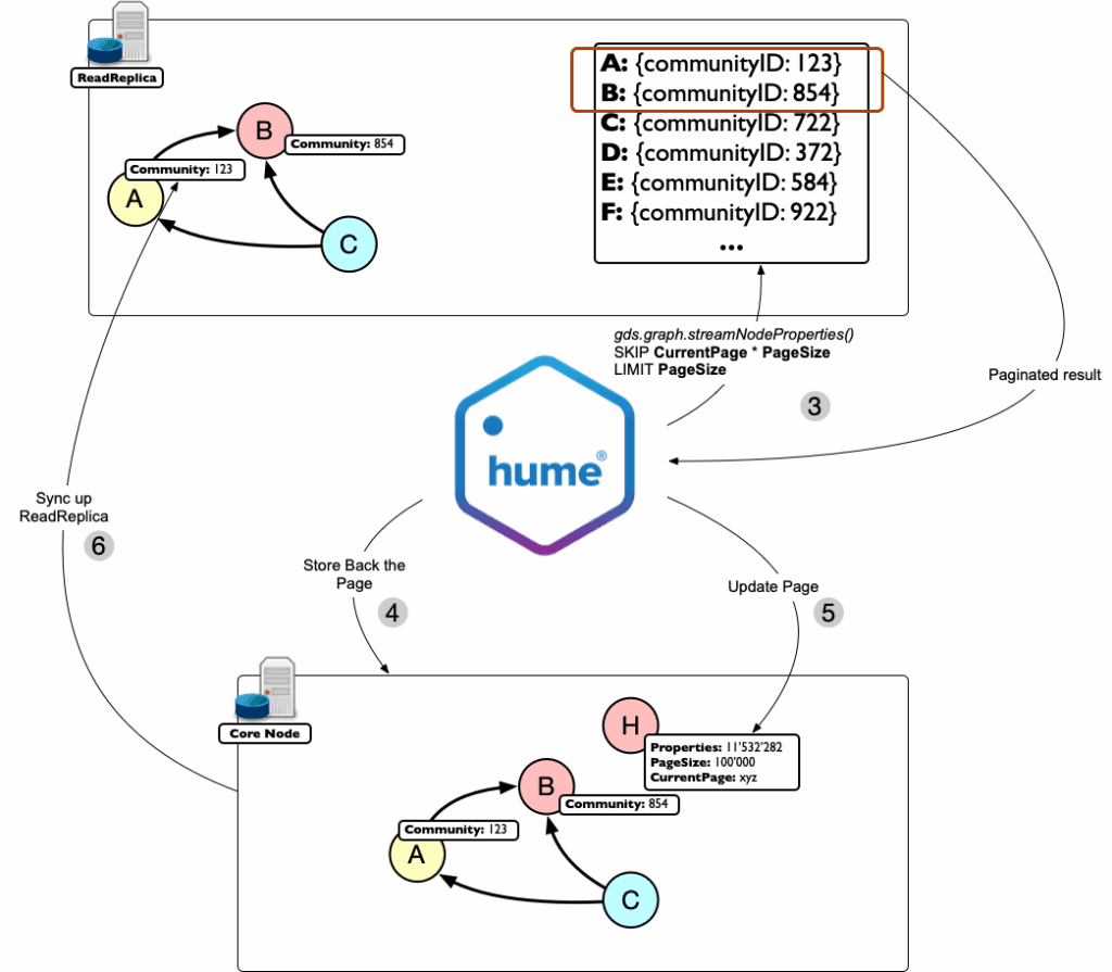
- We then iteratively fetch one “page” at a time using the gds. graph. The streamNodeProperties function, in combination with a SKIP/LIMIT clause, effectively selects one page worth of data at a time.
The actual “store back process” now consists of:
- Updating the relevant nodes with the communityId property as usual,
- Updating the PagingHelper node by incrementing its CurrentPage property and
- Updating Read Replica (the cluster will automatically synchronise the replica for us).
By comparing the PagingHelper node’s properties, such as CurrentPage, PageSize, and Properties, we always know whether the process is completed or not.
If this sounds complex to you at first glance, you will be surprised by how it fits nicely in a couple of workflows:
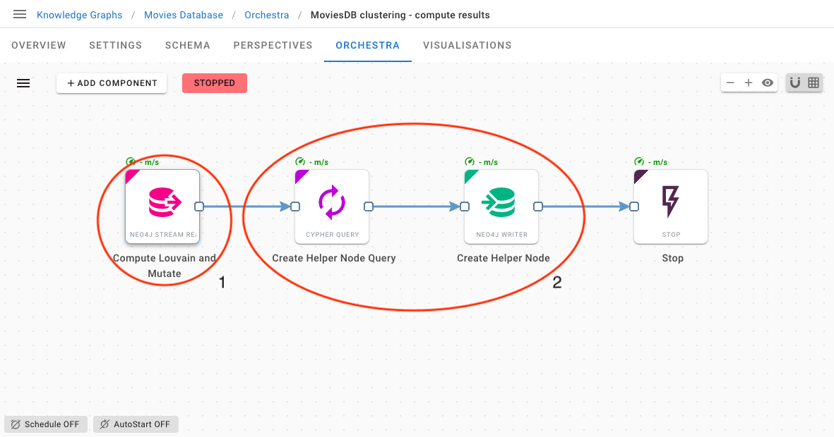
Again, by leveraging the ability of Hume to mix and match multiple resources, it is easy to implement steps (1) and (2)
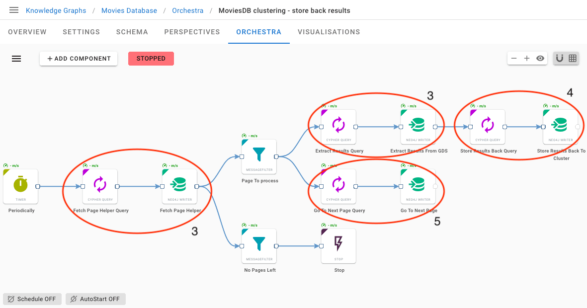
Here we start by periodically fetching the current page information from the helper node. Using this information, we select the portion of output to extract (3) and store that portion back (4).
At the same time, we update the helper node (5) and let the workflow iterate through this process until there is nothing left to do, which triggers an automatic stop of the whole workflow.
Conclusions
Graph data science is playing a crucial role in many businesses, and it will become even more prominent in the future.
Neo4j’s GDS library is a central technology in this area, where real-life applications keep requiring the computational support that only cluster configurations can give.
We showed how to tackle the Account Association problem in a realistic setting where it is essential to decouple Core nodes and Computational nodes.
We also saw that, while it is easy to move data in one direction, it is not apparent how to synchronise results back, and we proved how GraphAware Hume fills the gap at scale.
This is how GraphAware Hume allows you to focus on your data processing and analysis logic, making it easier for you to bring value to your business.

