Welcome back to the Graph-Powered Machine Learning book club. Now we are in the section of the book that focuses on recommendations. In the last blog, I summed up how content-based recommendations work. In the fifth chapter, the author Alessandro Negro introduces us to collaborative filtering.
From this blog, you’ll get insights into:
- What is collaborative filtering
- How to provide recommendations with collaborative filtering
- What is the cold start problem, and
- How can you solve the cold start problem with graphs.
Ready to dive in?
What is collaborative filtering?
Collaborative filtering is the most common technique to provide more accurate recommendations than the content-based approach. It uses past user behaviour (clicks, purchases, ratings) to predict items of interest. Thus, this approach does not need information about items to provide recommendations.
There are two paths you can take to find the items of interest to the users:
- Memory-based neighbourhood methods. These focus on the neighbours of items or users.
- An item-based approach predicts the user rating of an item based on his/her ratings of similar items.
- User-based approach finds similar users and recommends the items they liked. In memory-based methods, the user-item dataset is used directly to provide recommendations.
- Model-based methods. These methods create models for users and items. These models consist of relevant features and the weights for these features. The raw user-item dataset thus first needs to be processed offline to create the models. Only the created model is needed to provide recommendations during the recommendation phase.
The chapter focuses on neighbourhood-based methods. These methods have several advantages over the model-based ones:
- They have a level of serendipity. The recommendations provided by the user-based approach can be more diverse.
- They are simpler. Compared to model-based methods, fewer (sometimes only one) parameters require tuning.
- They are justifiable.
- They are efficient. Neighbourhood-based methods provide near-real-time recommendations. Storing only the nearest neighbours saves space, making the approach fast and scalable.
- They are stable. Adding more data affects the performance only very slightly.
- They are graph-based. The nearest neighbour model can be stored in a graph. Doing so makes it easier to navigate the model and access the data. It also helps tackle the cold start problem (discussed later).
Providing collaborative filtering recommendations
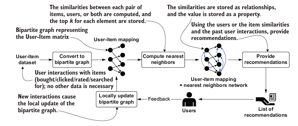
The collaborative filtering approach needs only the record of past user interactions. Let’s walk through how to provide a collaborative filtering recommendation step by step:
- Convert the user-item matrix into a bipartite graph.
- Compute similarities and create a nearest neighbour network.
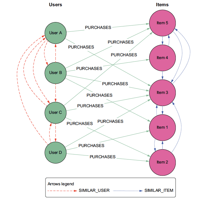
- Store the top k neighbours back into the (no longer bipartite) graph. Store the levels of similarity as properties on a relationship, assigning them weights.
- Run a graph-matching query combining previous user interactions and nearest neighbours. The results are your recommendations.
- New interactions enrich the original graph, updating the model. This allows for relevant recommendations to be served even when people’s tastes change.

Now let’s dive into each of these steps a little more.
Creating a bipartite graph for the user-item dataset
Collaborative filtering is based on user interactions with items – a user-item dataset. This dataset can be represented in a bipartite graph (bi-graph), with a set of users and a set of items. The bipartite graph has relationships only between nodes of different sets.
From this bi-graph, we can infer two one-node projections. One will show the relationships among users, and the other the relationships among items. Such projections, however, hide a lot of information from the original bi-graph. For instance, they don’t show how many users bought the same items. To solve this, you can add a weight property to the relationships. You can also use clustering algorithms to surface more information in the graph. These algorithms can identify user segments or items that are commonly bought together.
The bipartite graph representation is useful because:
- It is compact and intuitive.
- The one-node projections inferred allow for further graph or algorithmic analysis.
- It allows a nearest-neighbour network to be computed. Such a network is a great basis for providing recommendations.

Computing the nearest neighbour network
The item-based approach computes similarities between items purchased by the same users. In the user-based approach, the similarities are computed between users purchasing similar items.
The process for similarity computation is the same as for the content-based approach:
- Identify a similarity function you want to use.
- Represent each element (item and user) to prepare it for the similarity computation.
- Compute similarities between homogeneous items – nodes of the same class.
- Order the similarity values from high to low.
- Keep the top k similarities in a graph.
The final step results in a non-bipartite graph. Out of this graph, you can create 3 subgraphs:
- Graph with both items and users.
- The nearest neighbour network for users. Applying clustering algorithms to this network helps you identify segments of similar users.
- The nearest neighbour network for items. By applying clustering algorithms here, you can identify items bought together. You can also find items similar to a specific product.
Providing recommendations
Recommendations are made based on relevance scores between items and users. Relevance scores predict how much a user will like a particular item. They are based either on the nearest neighbour network of users or items.
To find the nearest neighbours of a user, you need to compute similarities for each pair of users. The same applies to finding item neighbours; however, this is generally faster. There are probably fewer item pairs in your database than user pairs. Take the example of a movie streaming platform.
There are thousands of movies available to watch for millions of people. It’s impossible to compute similarities between all the user pairs in real time. Thus, the user-based approach is not suited to compute recommendations in real-time. The item-based approach requires fewer similarity computations and thus can provide real-time recommendations.
The cold start problem
As you know by now, collaborative filtering relies on past user interactions. The problem appears when there is little or no data available about past interactions. This is the case with new users, who have not interacted with many items.
How can you provide valuable recommendations to these users? There are several approaches to solving the cold start problem. One solution is to build a hybrid recommender system. Such a system solves the issue by using other kinds of data in addition to the past user interactions.
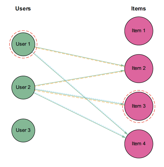
Graphs also provide a solution to the cold start problem. Generally, the length of a path between a user and an item in collaborative filtering is 3.
Here is how the path looks in the user-based approach:
- User 1 purchased item 2
- Item 2 was also purchased by user 2
- User 2 also bought item 3 – item 3 is recommended to user 1

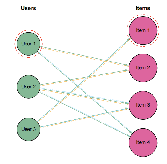
To solve the cold start problem, you can focus on longer paths – indirect associations – as well. Paths of length 5 provide more recommendations to the users:
- User 1 purchased item 2
- Item 2 was also purchased by user 2
- User 2 also purchased item 3
- Item 3 was also purchased by user 3
- User 3 also purchased item 1 – item 1 is also suggested to user 1

The longer the path, the more recommendations you can make. This solution is simple and effective as it uses the same bipartite graph. Even so, using indirect associations decreases the recommendation quality.
Conclusion
Collaborative filtering is the most commonly used approach to providing recommendations. It relies on past user interactions with items. Thus, it can provide recommendations when you don’t have information about items.
The user-item dataset can be easily represented in a bipartite graph, with two sets of nodes: user and item nodes. The bipartite graph uses less space as it stores only relevant/existing relationships. You can infer two one-node projections from the bi-graph. These projections show the relationships among the nodes of the same class.
The result is a k-nearest neighbour network showing the top k neighbours of items/users. K-NN is a basis for recommendations, and/or further graph and/or algorithmic analysis.
The cold start problem occurs when there is a limited amount of data on past user interactions. Graphs can solve this problem by taking longer paths to provide recommendations. Thus, graphs provide a well-rounded solution for collaborative filtering models. Visit our detailed collaborative filtering glossary page for more information.

