Introduction
In the bucket-filling problem, you are given two empty buckets, each of a certain capacity, and a large supply of water. By filling, emptying and transferring water between the two buckets, you must try to end up with a situation where one of the buckets contains a required volume of water, or where both buckets together contain the required volume.
One popular instance of the problem has two buckets with a capacity of 5 and 3 litres respectively, with the goal being to find a solution where one bucket contains exactly 4 litres. One solution is shown below:
| Transfer water to a 3-litre bucket | Action | Bucket volumes (5l, 3l) |
|---|---|---|
| 1 | Fill 5 litre bucket | (5, 0) |
| 2 | Transfer water to 3 litre bucket | (2, 3) |
| 3 | Transfer water to a 3-litre bucket | (2, 0) |
| 4 | Transfer water to 3 litre bucket | (0, 2) |
| 5 | Fill 5 litre bucket | (5, 2) |
| 6 | Transfer water to 3 litre bucket | (4, 3) |
One of the interesting features of this problem is that if the bucket capacities are relatively prime, it is always possible to find at least one solution for every integral volume of water, up to the combined capacity of the two buckets. Solving the problem is not too hard to do in your head when the bucket capacities are fairly small, but as they get larger, it gets exponentially more difficult.
Solving the problem with a graph
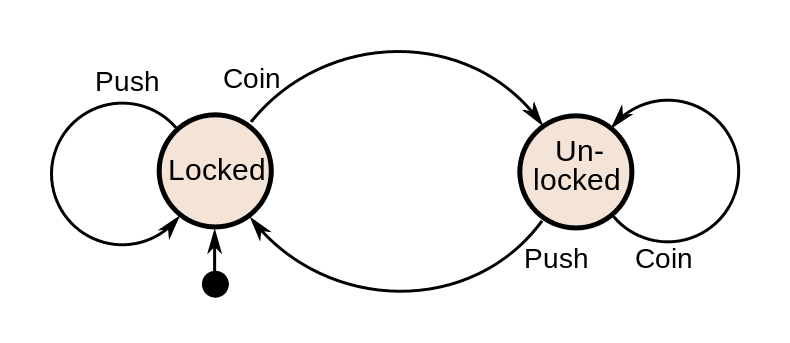
To solve the problem using a graph, we can model it as a state machine. A state machine is an abstract representation of a dynamic system in which every possible state the system can be in is uniquely represented, and the means by which the system can transition from one state to the next are also fully enumerated. This diagram from Wikipedia shows how the behaviour of a turnstile can be represented as a state machine:

From a graph perspective, every state in a state machine is a node, and every transition is an edge connecting exactly two nodes. So we can define every possible permutation of the bucket volumes as the nodes in a graph, and the actions of filling, transferring and emptying water as the edges connecting them. The first step is therefore to create the nodes.
Creating the nodes
We create BucketPair nodes with two properties, m and n, representing the volumes of water in each bucket. Given two initial bucket capacities {m, n}, this will result in m x n nodes.
Note that in this example, I have chosen initial bucket capacities of 13 and 7, but you can use any values you like
MATCH (bp:BucketPair) DETACH DELETE bp
WITH [13,7] AS values
UNWIND range(0,values[0]) AS m
UNWIND range(0,values[1]) AS n
MERGE (bp:BucketPair {m:m, n:n, name: "(" + m + "," + n + ")"})
After the state nodes have been created, the next step is to create the edges representing the permitted state transitions between them.
I have chosen to use an ACTION edge for all the transitions, with a name property to distinguish them, but you could also use different edge types instead.
Fill
The Fill action is permitted if any BucketPair node has an empty bucket, indicated by either its m or n property being 0. An ACTION edge with the name Fill links this node to the one representing the empty bucket being filled. For example, given initial bucket capacities of (5, 3), we would create a Fill edge between the BucketPair nodes (0, 3) and (5, 3).
WITH [13,7] AS values
MATCH (s:BucketPair {m:0})
MATCH (t:BucketPair) WHERE t.m=values[0] AND t.n = s.n
MERGE (s)-[:ACTION {name:'Fill'}]->(t)
WITH values
MATCH (s:BucketPair {n:0})
MATCH (t:BucketPair) WHERE.n=values[1] AND t.m = s.m
MERGE (s)-[:ACTION {name:'Fill'}]->(t)
Transfer
This action represents pouring as much water as possible from one of the buckets into the other. The target of a transfer edge in the graph is therefore the node representing the state of the buckets after the water has been transferred. There are some rules: obviously, water cannot be transferred from buckets that are empty, or into buckets that are already full. Most importantly, you aren’t allowed to partially fill a bucket if you can fill it completely. There are many potential partial transfers of water between buckets that are not allowed by the rules of the problem, and we need to make sure we don’t create edges for the illegal ones.
Rather than laboriously checking through all of the possibilities to find the only correct one, we can use a little trick. First, we find all the nodes representing all transfer candidates from a particular node. (A candidate BucketPair is one where the total value of water in the buckets is the same as the one we’re transferring from). This will, of course, include many partial transfers, which are illegal as noted above. Each of these candidates has an m and an n value. A little thought should hopefully reveal that the smallest m value combined with the largest n value from among these candidates must be the volumes for the only legal transfer, so we simply need to find the BucketPair node with those volumes and create an edge to it:
WITH [13,7] AS values
MATCH (s:BucketPair)
MATCH (t:BucketPair)
WHERE t.m + t.n = s.m + s.n // we can't lose/gain water
AND NOT t = s               // we can't transfer to the same node
AND s.n < values[1]         // we can't transfer into a full bucket
AND s.m > 0                 // we can't transfer from an empty bucket
WITH s, min(t.m) as m, max(t.n) as n // identify target (m, n)
MATCH (t:BucketPair) where t.m = m and t.n = n
MERGE (s)-[:ACTION {name:'Transfer'}]->(t)
Empty
Any bucket containing water can be emptied, so implementing this transition in the graph simply involves finding each non-empty bucket and creating an edge from it to the corresponding node representing that bucket being empty.
MATCH (s:BucketPair) WHERE s.m > 0
MATCH (t:BucketPair) WHERE t.m = 0 AND t.n = s.n
MERGE (s)-[:ACTION {name:'Empty'}]->(t)
WITH 0 AS dummy
MATCH (s:BucketPair) WHERE s.n > 0
MATCH (t:BucketPair) WHERE t.n = 0 AND t.m = s.m
MERGE (s)-[:ACTION {name:'Empty'}]->(t)
A quick look at the graph
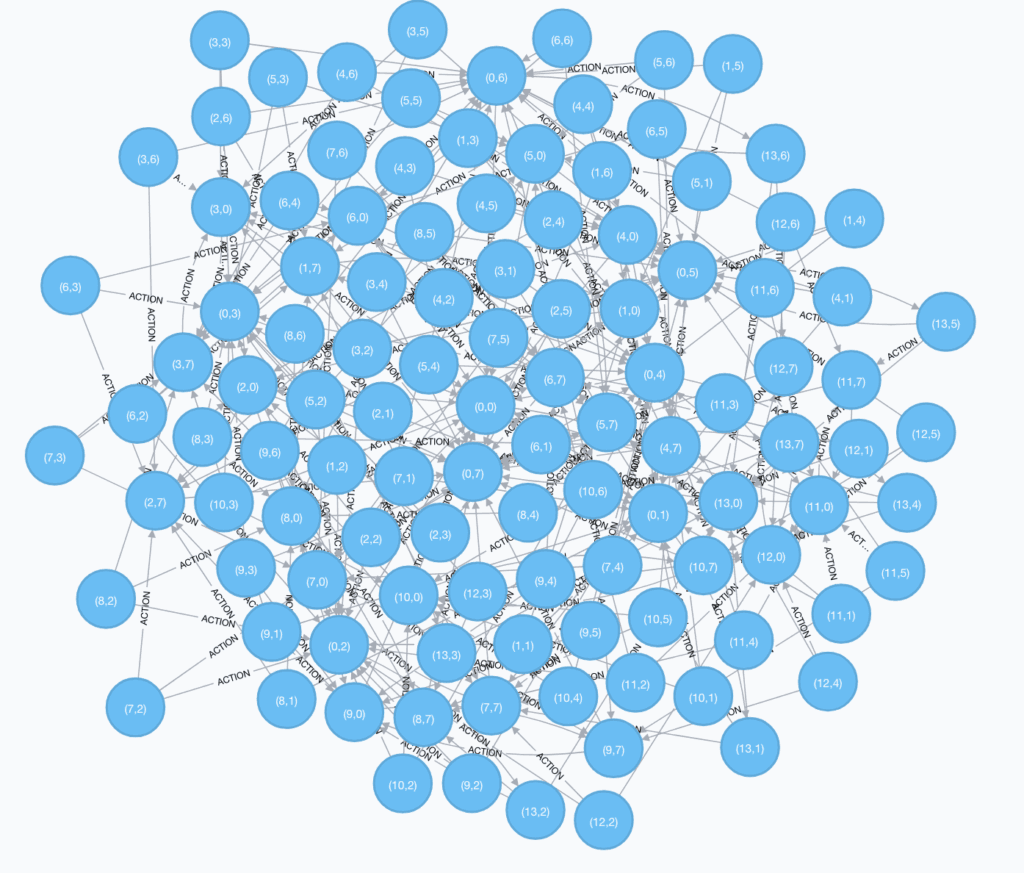
It is interesting to see what this graph looks like after we create it. Using the two bucket capacities used above (13,7), we end up with a graph containing 122 nodes, 22 Fill edges, 202 Empty edges and 91 Transfer edges.

As you can see, it is a fairly dense structure. The number of paths is huge: if you wanted to find a solution for a quantity of 14 litres, you probably couldn’t do it in your head – it requires 35 steps.
An optimal solution = a shortest path
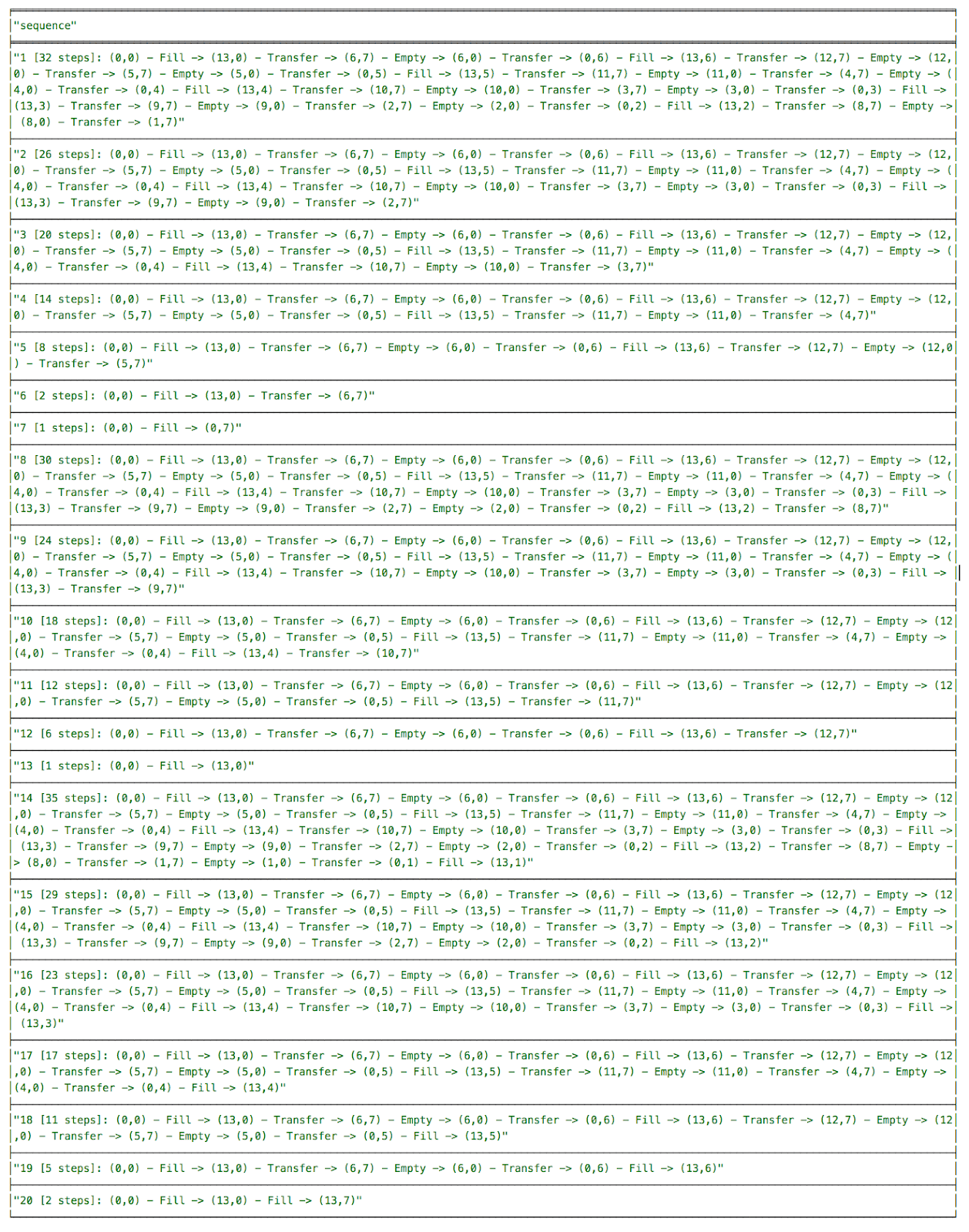
Thankfully, now that we have a graph, we don’t have to torture ourselves to find solutions. We can use Cypher’s shortest path algorithm to do it for us, which will quickly find an optimal solution for any feasible volume of water. Here’s the Cypher to generate all solutions for the initial bucket capacities of (13, 7)
WITH [13,7] AS values
WITH values, range(1, values[0] + values[1]) AS qs
UNWIND qs as q
MATCH (s:BucketPair) WHERE s.m = 0 AND s.n = 0
MATCH (t:BucketPair) WHERE t.m = q OR t.n = q OR t.m + t.n = q
MATCH paths = shortestPath((s)-[:ACTION*]->(t))
WITH q, paths ORDER BY length(paths)
WITH q, collect(paths) as paths
WITH q, paths[0] AS path,
extract(n in nodes(path[0]) | n.name) AS buckets,
extract(r in relationships(path[0]) | r.name) as actions
RETURN q + " [" + size(actions) + " steps]: Start -> " + head(buckets) +
       reduce(acc = "", i in range(1,size(actions)) |
              acc + " - " + actions[i-1] + " -> " + buckets[i]) as sequence
ORDER BY q
And here are the results

Fun fact
Earlier, I mentioned that if the bucket capacities are co-prime, there is a solution for all integral volumes of water up to the combined capacity of the buckets. However, if the capacities are not co-prime, this is not possible. In fact, we can only ever obtain solutions for volumes that are some multiple of the greatest common divisor of the two bucket capacities. So it is only because gcd(a, b) = 1 when a and b are co-prime that we are able to get solutions for all volumes. If you’re interested in knowing more about this, check out Bezout’s identity
Conclusion
Graph databases are an excellent technology for representing optimisation problems that can be solved using path-finding techniques. This simple example illustrates a graph-based approach that you can consider using for other optimisation and decision problems representable as state machines, where search can be used to find a solution. Some examples that spring immediately to mind are health and vehicle diagnostics, process verification, routing decisions and language parsing – I’m sure you can think of others.
