Building & exploring a music knowledge graph

It is always a valuable opportunity to understand our product better and recognize user needs. At GraphAware, building Hume, a graph-powered insight engine, we are proud of making an impact on our customers’ success. However, we use Hume also to support our processes and help our own needs. In the case of the event that took place throughout December, we were also able to have great fun and integrate the team.

Challenge

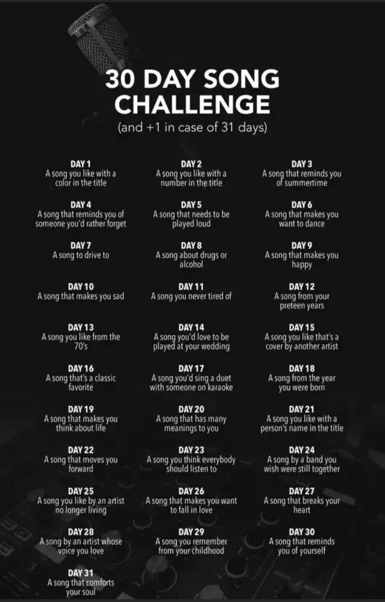
Have you heard about the 30 Day Song Challenge? This is a game that cheered us up on short European December days. Every day we proposed songs on Slack according to a new theme. In this way, we collected almost 400 songs in various categories.

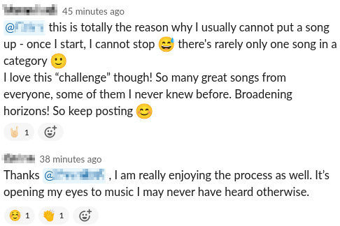
The game was well received, and it was met with a good response from the team.

We realised that creating a database of our music tastes would be interesting and fun. Having enriched it from different data sources, our data science engineers will open almost limitless possibilities for analysis. As a result of the experiment, we can build an interesting knowledge graph that can be an exciting experiment for exploring the capabilities of Hume.

Importing data

As we are a graph-aware company, there were no second thoughts to import data into Neo4j and build a new knowledge graph in Hume. Thanks to regular and intense activity of Luanne, using the “physical protein interface,” we collected data in the Google spreadsheet. The first Orchestra pipeline we built was regularly reading the spreadsheet and ingesting data into Neo4j.

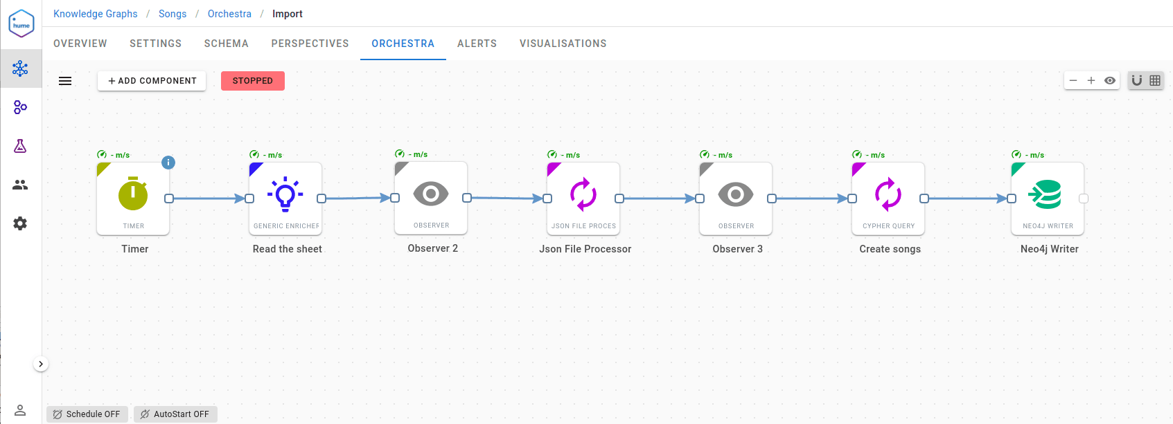
The workflow is straightforward. The timer component triggers the data pipeline periodically every 30 minutes, and Generic Enricher component fetches spreadsheet data using Opensheet API. Then a response is transformed using the Json File Processor component, and it is used as the input for creating a cipher query. Finally, every song is stored in the Neo4j database.

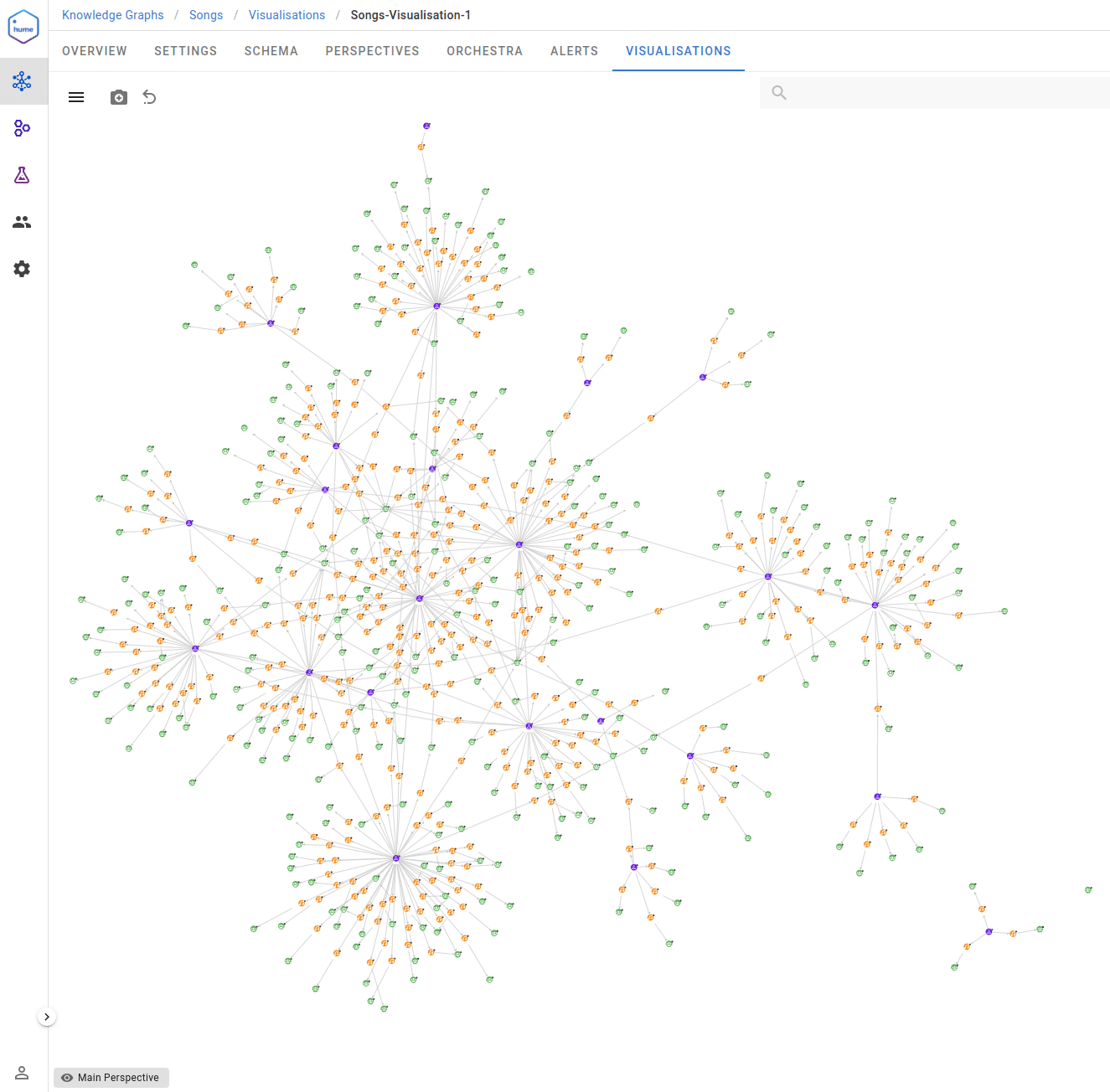
Very quickly, we could see our first music song graph. Our imagination has exploded at this point.

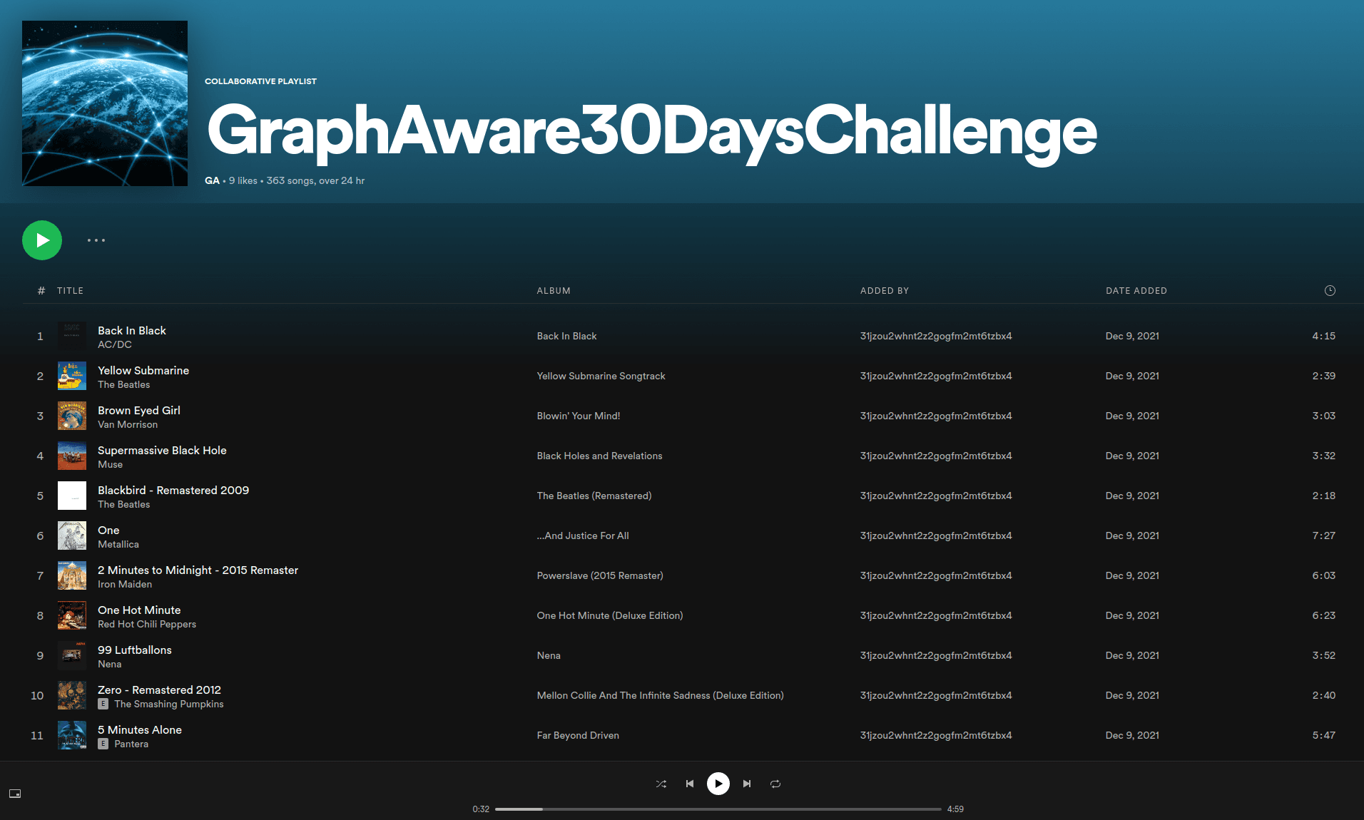
Spotify playlist

Keeping in mind that we are building a music knowledge graph, we realised it’s time to prepare for New Year’s eve and create a Spotify playlist. The Spotify API is very well documented so a new workflow was created quickly:

Neo4j is the source and the target database for workflow data processing. First, the workflow reads songs provided by participants (i.e., without Spotify’s identifier), and at the end, it enriches the songs in the graph with additional information.

Three major points of the workflow are Generic Enricher components that use Spotify API in order to complete the following tasks:

• Find a song in Spotify’s database and retrieve its URI
• Get existing playlist content
• Add new tracks to the playlist

Message Transformer components make sure JSON documents processed by the pipeline are correctly transformed using Python scripting. This is one of the features that every data scientist/engineer will surely find essential. In order to improve the performance, it uses a Batch Processor that allows aggregating a stream of messages into a single message of defined size. When the job is done, and all songs are analysed, the Idle Watcher component is triggered, stopping the workflow.

Finally, we were able to build and share our first GraphAware playlist with the world, which consists of more than 360 songs and is over 24 hours long.

Data enrichment from external services

Are you already excited as we were? Because it’s just the beginning of the story.

Neo4j is a schema-free graph database. Therefore, it’s very easy to expand and enrich our database with data obtained from other structured data sources, thus starting the process of transforming an ordinary graph into a Knowledge Graph.

We enriched the graph with additional data:

• Song genre information (iTunes, Wikidata)
• Album name and track number (iTunes)
• Artist’s birth date and inception date (Wikidata)
• Who the artist is inspired by (Wikidata)
• Song tempo or beats per minute (BPM) (Spotify)

In order to ingest such information, another set of workflows was built similarly to the previous one. Here, the advantage of having an orchestration tool really shines: with the low coding effort, we can build a robust fault-tolerant pipeline just from a UI interface.

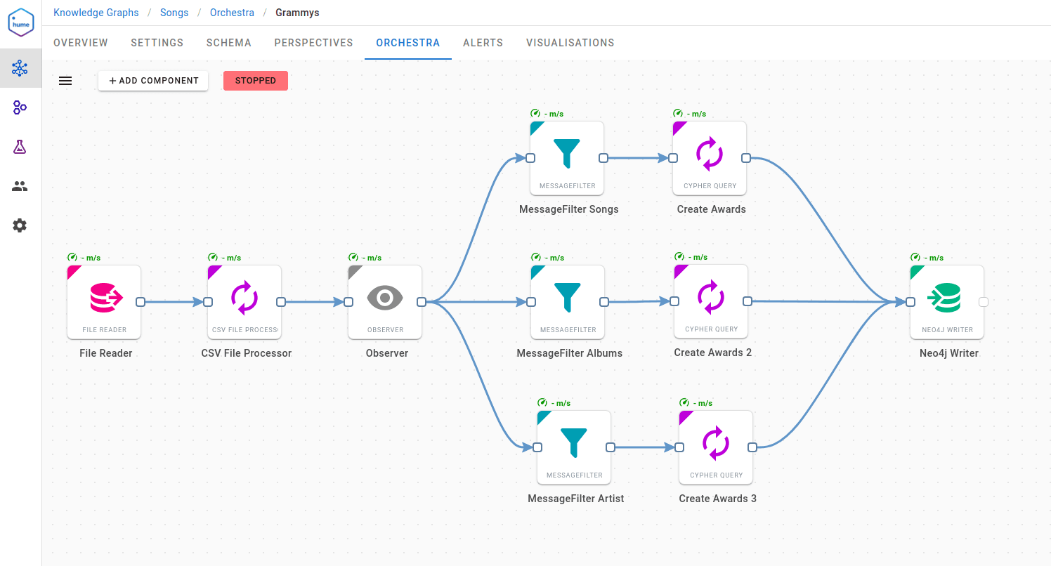
Grammy awards

We wanted to know how fans and the music industry recognized songs. Therefore, the next step was to supply information about the Grammy Awards. As you may have already guessed, another simple workflow did the job. This time we extracted data from a CSV file located in our blob storage, containing a public dataset of Grammy Awards.

It’s a good opportunity to mention what kind of data sources are supported by Orchestra. The list is impressive. It supports:

• all SQL databases (using JDBC connector)
• no SQL data sources (Neo4j, Mongo)
• messaging systems (Kafka, RabbitMQ)
• local and cloud file systems (AWS S3, Google Storage)
• web APIs (RSS feed, web hook)

Finally, we were able to get completely new view of our data:

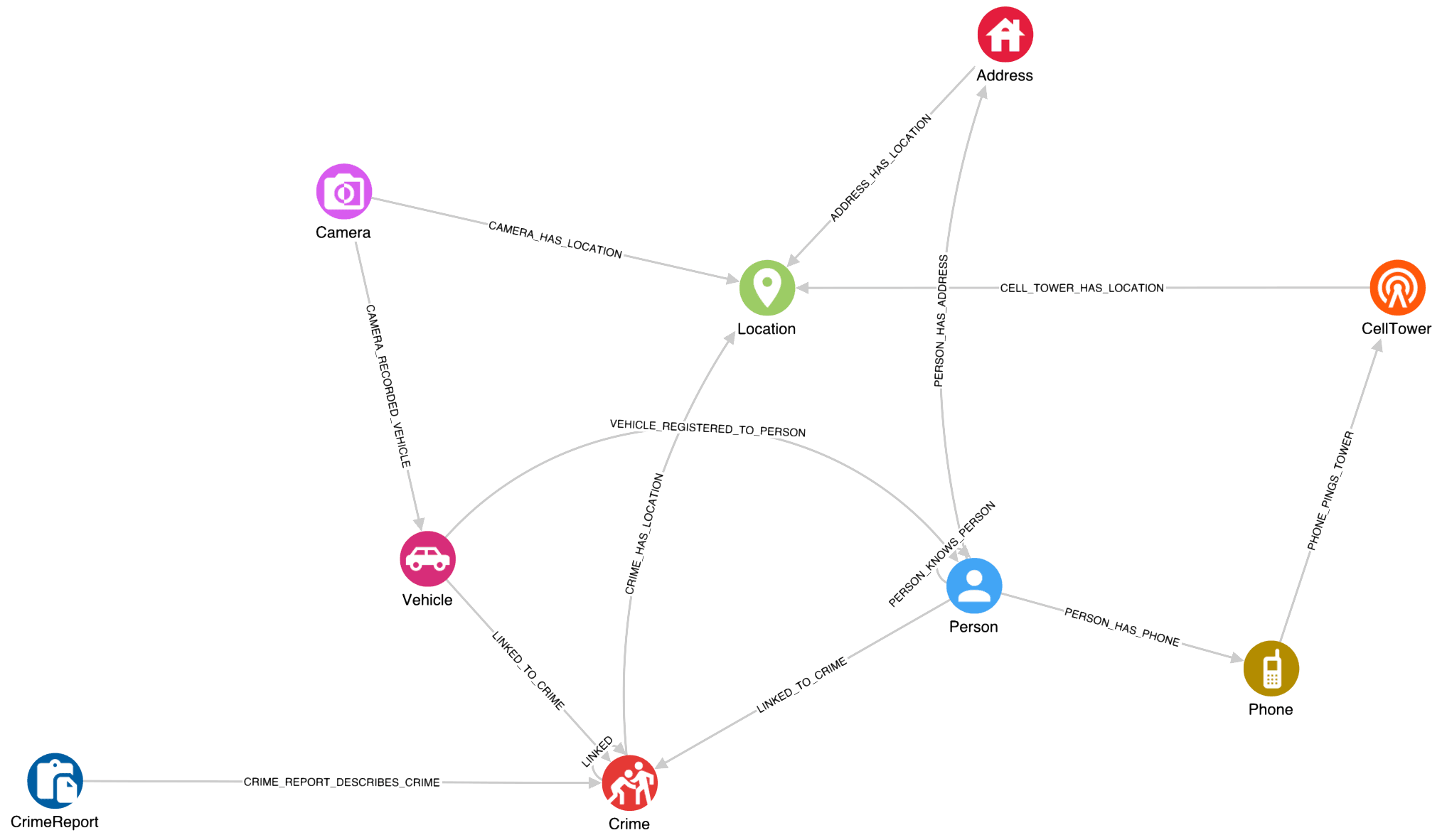
Fully enriched Knowledge Graph

After all the imports and enrichments, we reached the Knowledge Graph schema visualised below. The central point is the Song node, which has an incoming SHARED relationship from the Person who shared the song. Artists further produced Songs, and they have a Tag that represents the theme of the day suggested by the challenge. The rest of the graph results from knowledge enrichment from various sources, as described in the previous part. This way, we have gotten information about Genres, Albums, song Lyrics, how artists inspire each other, etc.

With all this in one central place, we can explore the connections and define analytical approaches to leverage all the collected information.

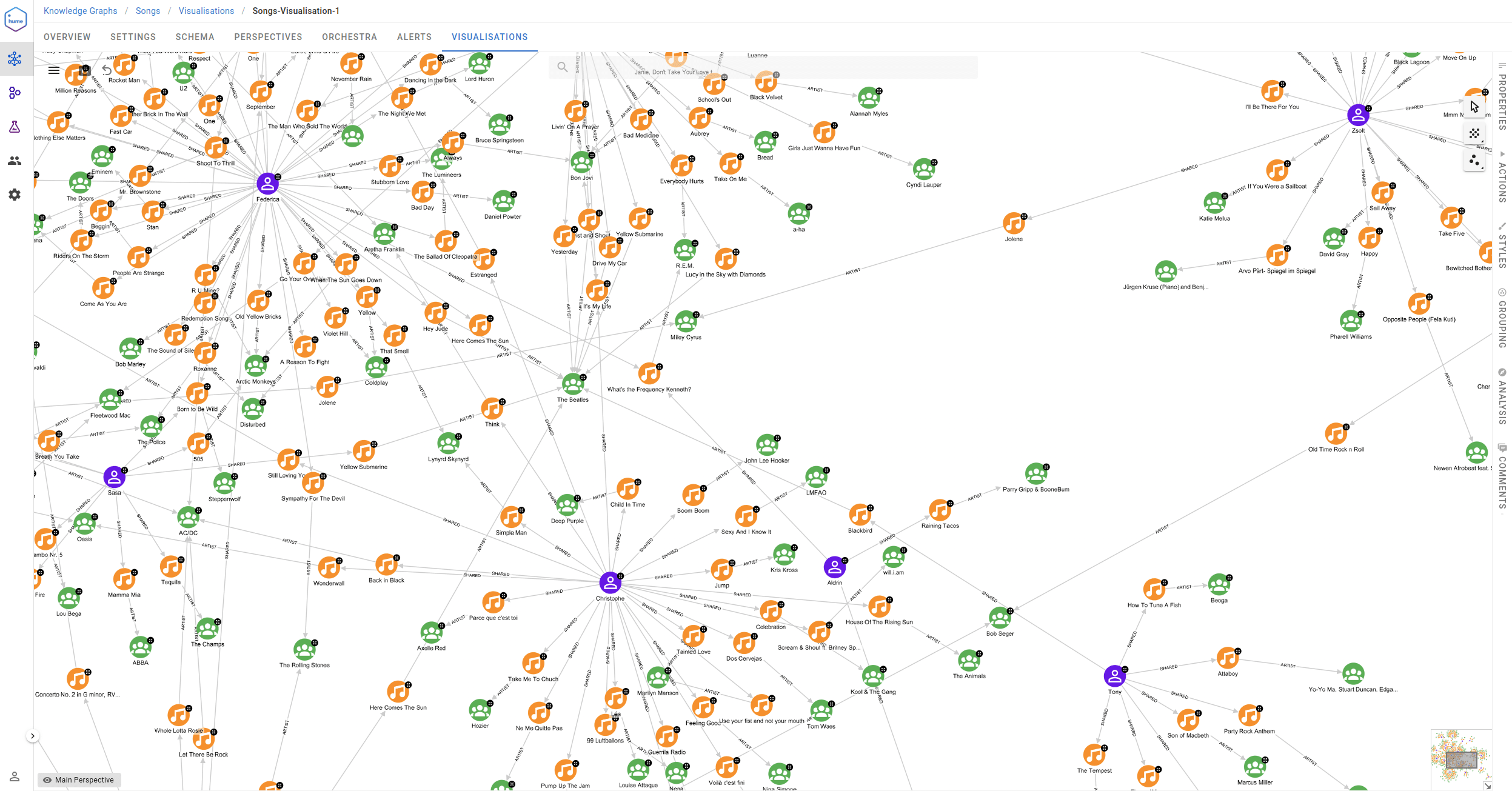
Find the most influential artists

An interesting exploration could be to search for the most influential artists in our network, based on the information gathered from Wikidata from the influenced by statements. Wikidata is a free and collaboratively developed structured knowledge base that is utilised for e.g. by Wikipedia. It can be read and edited by anyone following certain guidelines, which has both its pros and cons. The advantage is that it became a massive database containing various topics. On the other hand, not all the information is always 100% accurate. The artists’ influencers, for example, sometimes don’t have a stated reference supporting that fact, while other times it can point to a dubious source or uncertain statement such as “One source of inspiration might come from…”, yet it was entered into Wikidata as a fact. It is good to keep this in mind when interpreting the results we will be getting from our KG.

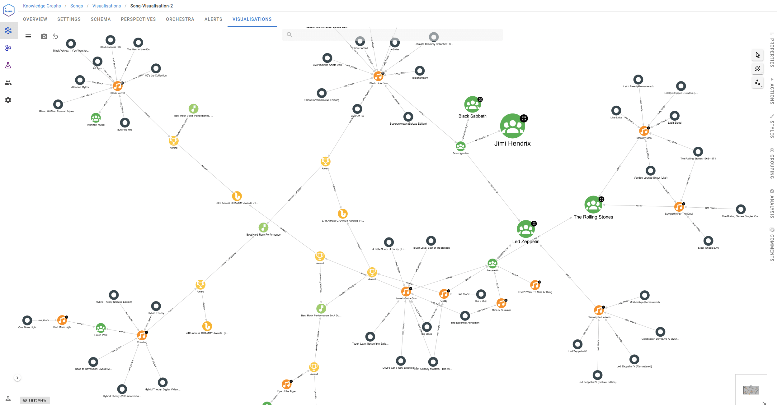
We used the PageRank centrality algorithm from the Neo4j GDS library to find the most influential artists. Based on each artist’s PageRank score, we created a visualisation style in Hume. This is what our artists’ graph looks like.

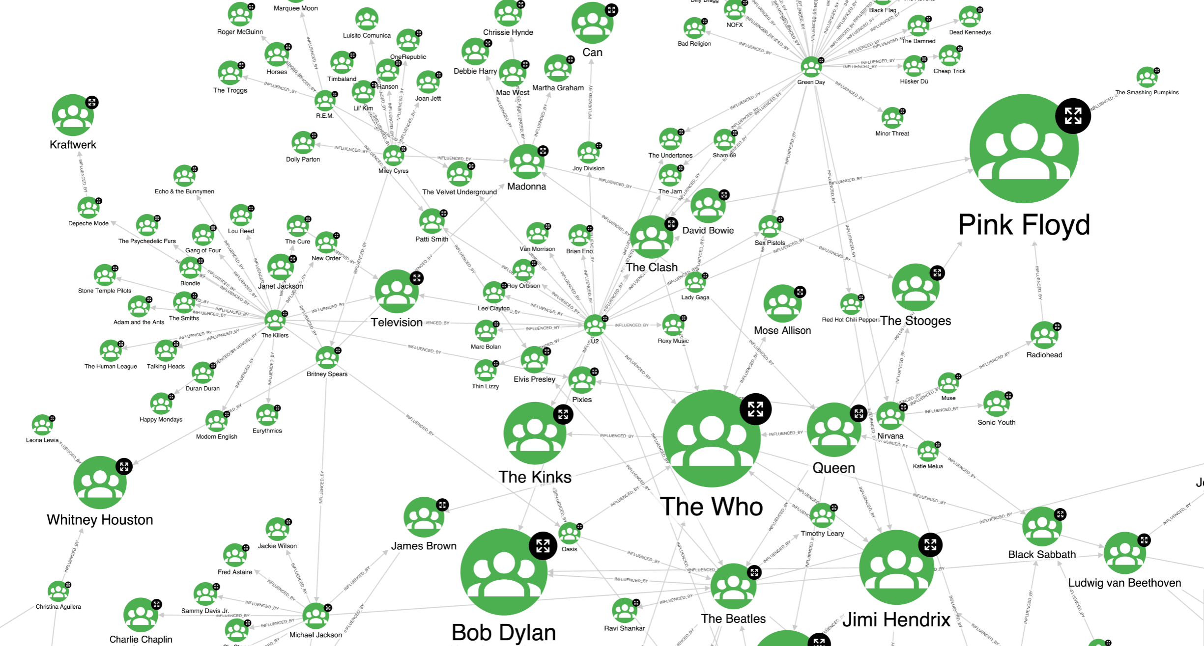
Google originally introduced PageRank algorithm to rank the importance of web pages for their search engine. It calculates the importance of each node by considering not only the number of incoming links but also their own importance. This way, nodes with a higher number of incoming INFLUENCED_BY relationships are identified as more central and have a higher PageRank score, hence a larger size in our visualisation. An example can be The Who which has 7 incoming edges. On the other hand, a node can be deemed important even when it has fewer incoming edges, but they come from nodes with high importance, such as Pink Floyd with 5 incoming links.

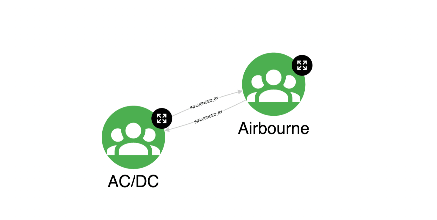
However, we arrived at the final result is not exactly straightforward, as sometimes PageRank may require some attention. It may happen that the algorithm gives too high scores to nodes that do not represent significant nodes from the centrality point of view. Indeed, this algorithm can behave strangely with so-called spider traps. For example, groups of isolated nodes with no link to the outside graph, or in a disconnected graph with multiple weakly connected components, where a component can be composed of only a handful of nodes with a cycle, as is visible in a screenshot below.

To overcome this problem, we decided to run the Weakly Connected Component (WCC) algorithm first, and then use PageRank only on the largest connected components. The WCC algorithm identifies sets of connected nodes in an undirected graph which are disconnected from the rest of the graph. For this reason this algorithm is often used at the beginning of the analysis to understand the structure of the graph and make sense of the results obtained by subsequent techniques. These are the Cypher queries used to obtain PageRank scores:

CALL gds.wcc.write( {
  nodeProjection: 'Artist', relationshipProjection: 'INFLUENCED_BY', writeProperty: 'wcc'} ) 
YIELD nodePropertiesWritten, componentCount
RETURN nodePropertiesWritten, componentCount

After running the WCC algorithm, we created a projection of our graph consisting only of nodes from the largest connected component. On this projection we applied PageRank:

CALL gds.pageRank.write( 'influence_Project', 
{writeProperty: 'pageRank', maxIterations: 200, dampingFactor: 0.85}) 
YIELD nodePropertiesWritten, ranIterations

It seems that for the GraphAware community, artists like Pink Floyd, The Who, and Bob Dylan are really influential. We wonder what it says about the average age of our company…

Community Detection

Another thing that attracted our curiosity was to find out how people in GraphAware could be grouped together according to their musical tastes. This, however, could be a complicated task. We need a measure of similarity between people to be able to cluster them together, but on the other hand we are dealing with a difficult task: songs are a combination of text (but careful - not always a nice straightforward natural language text, many songs have … let’s say a very “unique” lyrics ;) ) and music and often filled with various allusions, cues, sarcasm and emotion passed through a combination of music and lyrics which can shift the overall meaning.

Let’s look at the problem from a graph point of view. Looking at the schema, we notice that there exist connections among people through genres of their songs and artists. This is an important observation as it opens a way for assessing person-person similarity by the use of one of the graph metrics. Let’s start with creating helper relationships between Person and Genre, distinguishing between genres obtained from Wikidata and iTunes:

MATCH (n:Person)-[:SHARED]->(s:Song)
WITH n, count(s) AS total_shared
MATCH (n)-[:SHARED]->(s:Song)-[*1..2]->(g:Genre) WHERE g:FromWikidata 
WITH n, g, total_shared, count(DISTINCT s) AS num_genre
MERGE (n)-[r:WIKIDATA_GENRE]->(g) SET r.weight= toFloat(num_genre)/total_shared

In the same way, we worked with data from iTunes. Essentially, we created the WIKIDATA_GENRE relationship and assigned it a weight based on the ratio of shared songs or artists belonging to that genre. The reason why we split genres from the two sources is that we noticed that the data was not always the same, for e.g. David Gray’s Sail Away is classified as folktronica by Wikidata and singer/songwriter by iTunes, but both genres may be correct, it just depends on the criteria on which this classification is made. So to avoid confusion, we preferred to keep the information separate.

CALL gds.graph.create( 'genres_Weighted', 
['Person', 'Genre'], {WIKIDATA_GENRE: {properties: 'weight'}} )

With the query above we created an in-memory graph projection to calculate similarity between people based on the relationship just created. A similarity metric or measure quantifies the closeness between two items with respect to a particular property, in this case the “weight” property of WIKIDATA_GENRE. The measure we used is Node Similarity, which in turn uses the Jaccard Similarity Score. Jaccard is a useful measure for this application because it permits to consider the entire set of common elements between two nodes. This avoids comparing all genres of two people one by one, but takes into account common genres in relation to all the genres of the songs of the two people.

CALL gds.nodeSimilarity.stream( 'genres_Weighted', 
{degreeCutoff:1, similarityCutoff:0.23, relationshipWeightProperty:'weight'} )
YIELD node1, node2, similarity
WITH gds.util.asNode(node1) AS person1, gds.util.asNode(node2) AS person2, similarity
MERGE (person1)-[:SIMILAR_GENRE {genreSimil:similarity}]-(person2)

After that, we defined a new projected graph consisting only of Person nodes and relationships defined via Jaccard Similarity.

CALL gds.graph.create( 'genre_Similarity', 
'Person', {SIMILAR_GENRE: {orientation: 'UNDIRECTED'}}, { relationshipProperties: 'genreSimil'} )

Finally, we applied the Louvain algorithm to find communities of people. This is a hierarchical clustering algorithm that works by maximising a modularity score for each community. This modularity measures how much the nodes within a cluster are densely connected by assessing the number of edges within a community compared to the edges outside it.

CALL gds.louvain.write( 'genre_Similarity', 
{relationshipWeightProperty: 'genreSimil', writeProperty: 'louvainGenre'} )
YIELD modularity, communityCount 
RETURN modularity, communityCount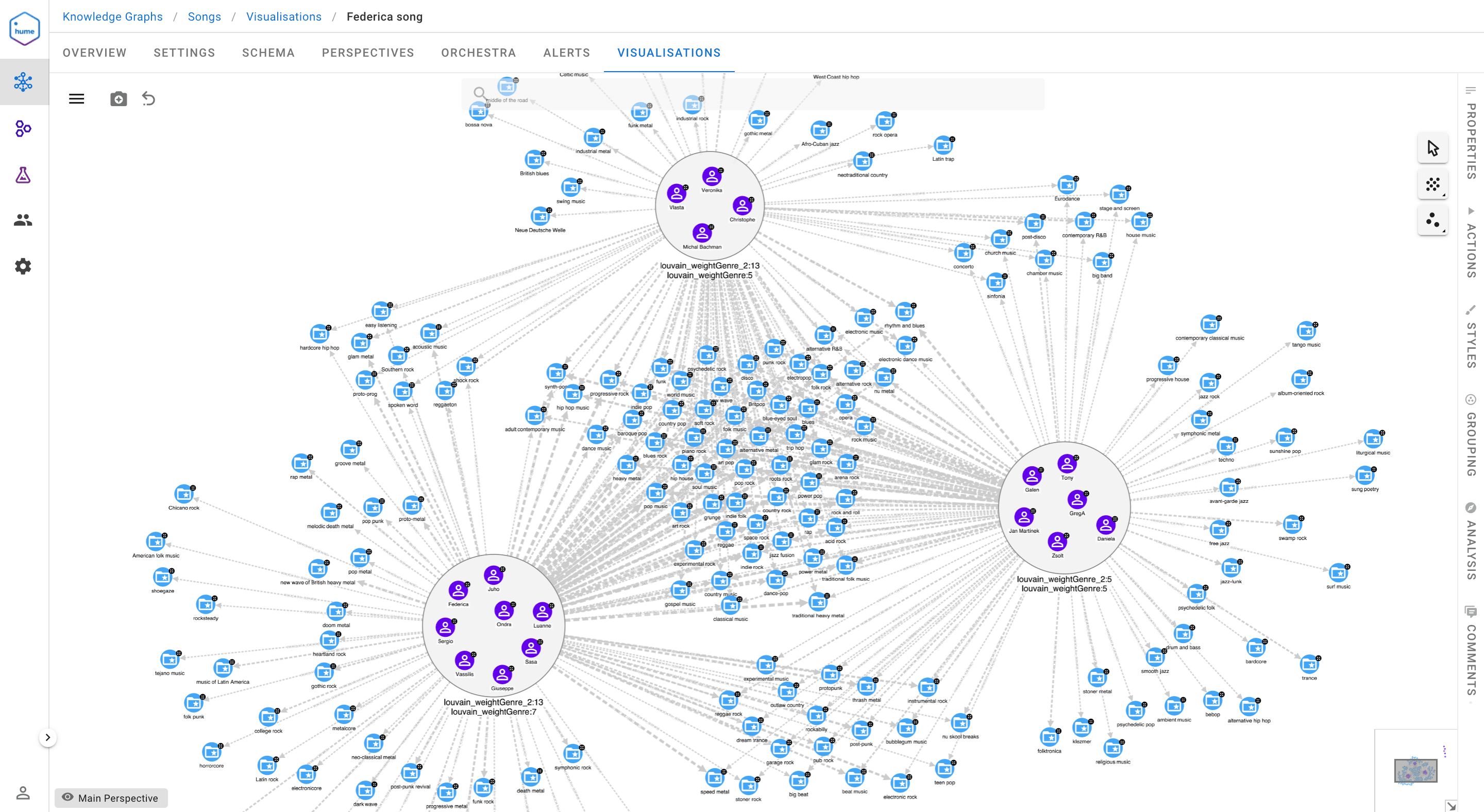

Observing the clusters obtained from the intersection of the communities from Wikidata and iTunes, we can clearly state that most people agree on rock; this genre is in the centre of our visualisation and is connected to all three largest communities. Moreover, the cluster on the left is composed of metal lovers, on the right we find people who like metal; and jazz, and at the top we have a mix of metal, electronic and blues.

A final remark concerns the way we appraised the resulting clusters. Obviously, the objective was to maximise the modularity of Louvain, but also to balance this value with the number of nodes that remained isolated. To achieve this goal, we investigated Jaccard’s “similarityCutoff” parameter, because this metric defines the relationships on which we eventually identify communities. Furthermore, we evaluated the clusters obtained with the help of the Conductance metric, which considers for each community the ratio between the relationships pointing outwards and the total number of relationships.

Songs suggestion

What if we wanted to suggest interesting songs to the lucky people who took part in the challenge? We identified the closest songs by defining the similarity between genres and BPM property. We applied Jaccard for the former and a similarity score based on the Euclidean distance for the latter. As one can imagine, there are a considerable number of similar metrics, and they work quite well, especially if we consider that they need only a few lines of Cypher code and do not need to be trained, so no data or time is required for this purpose.

Here is how we worked with BPM or tempo, by creating a SIMILAR_SONG_TEMPO relationship between all pairs of songs with a similarity of at least 0.11. We have chosen this value as threshold because this is the similarity obtained, using the formula below, for two songs with a BPM difference of 8.0, i.e. the smallest range of beats per minute between two distinct genres.

MATCH (s1:Song) WHERE EXISTS(s1.spotifyTempo)
MATCH (s2:Song) WHERE EXISTS(s2.spotifyTempo) AND s1<>s2
WITH s1, s2, 1.0 / (1 + abs(s1.spotifyTempo - s2.spotifyTempo)) AS similarity
WHERE similarity >= 0.11
MERGE (s1)-[:SIMILAR_SONG_TEMPO {tempoSimil: similarity}]-(s2)

Therefore, having all these similarity measures between people and songs, we had to create a Hume action to suggest songs. We wonder whether Juho likes our suggested songs…

Lyrics similarity

However, there are many other types of information that can be used and in this way it becomes possible to define other suggestion logics. For instance, we were able to import some lyrics, so we decided to focus our attention on keyword analysis, hoping to find songs about similar topics. Such an investigation is not too complex and does not require too much effort in Hume, as we have an unsupervised domain agnostic Keyword Extraction component readily available in Hume Orchestra. This is an algorithm that identifies and selects words or noun phrases that best describe a document. It was based on the TextRank algorithm and improved to also consider grammatical relations among tokens in selecting final multi-token keywords.

Once the keywords were obtained, we resolved to use SentenceTransformers, a Python framework that allows encoding sentences or paragraphs as dense vectors. With SentenceTransformers, we obtained semantically meaningful embeddings from our keywords. This means that the semantic relationship between keywords is preserved in their respective embedding vectors, so that two keywords that have similar meanings are mapped into nearby vectors in the embedding space. Lastly, we calculated the Cosine Similarity between the embedded keywords, another similarity measure particularly used in the NLP field, and searched for similar songs based on the similarity of their keywords.

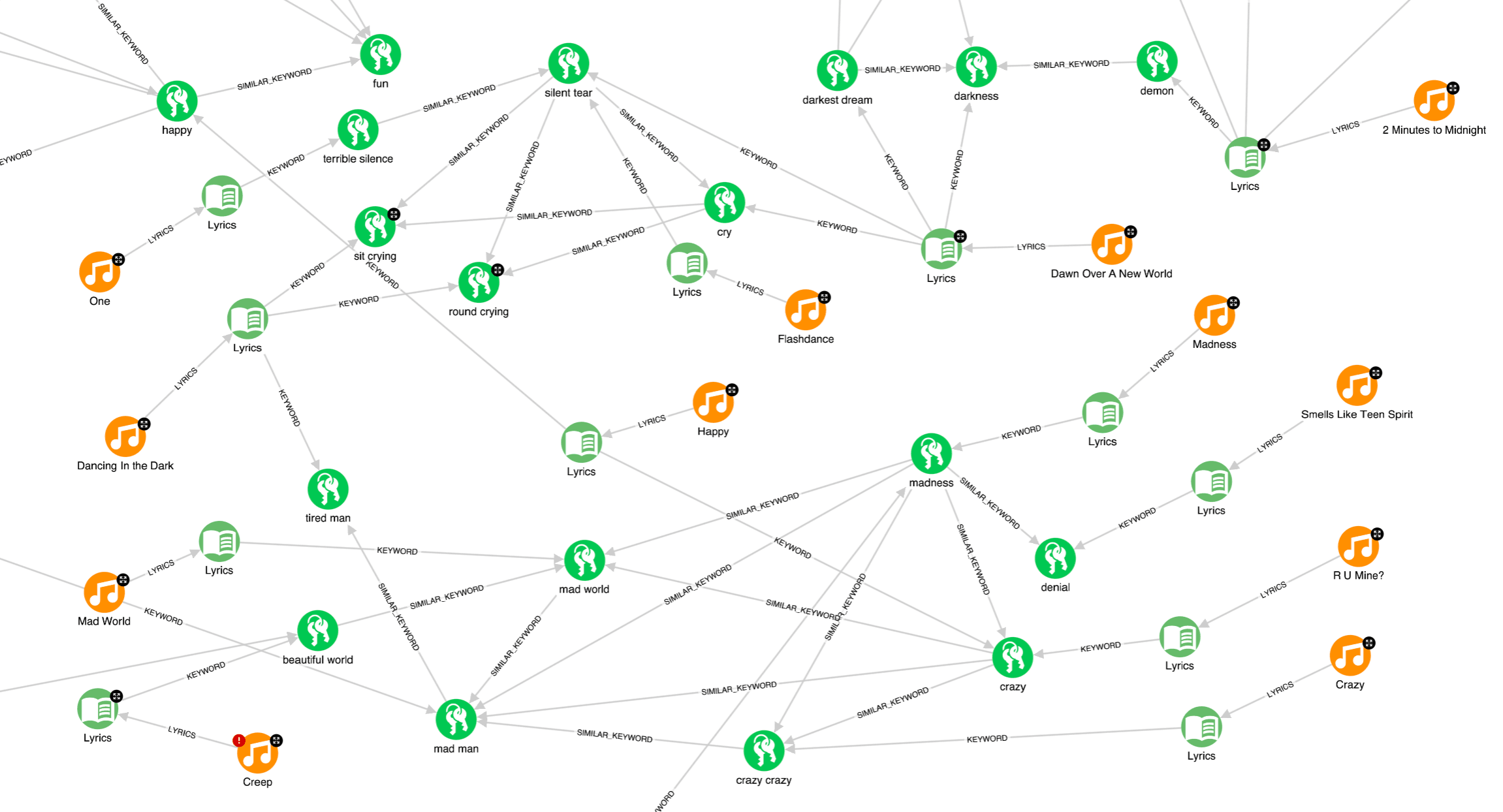
It seems that “Crazy” by Aerosmith has a similar keyword to “R U Mine?” by Arctic Monkeys. Gary Jules’ “Mad World” and “R U Mine?” also have similar keywords, both songs are about madness, but actually, with two different meanings… Quite challenging to work with lyrics.

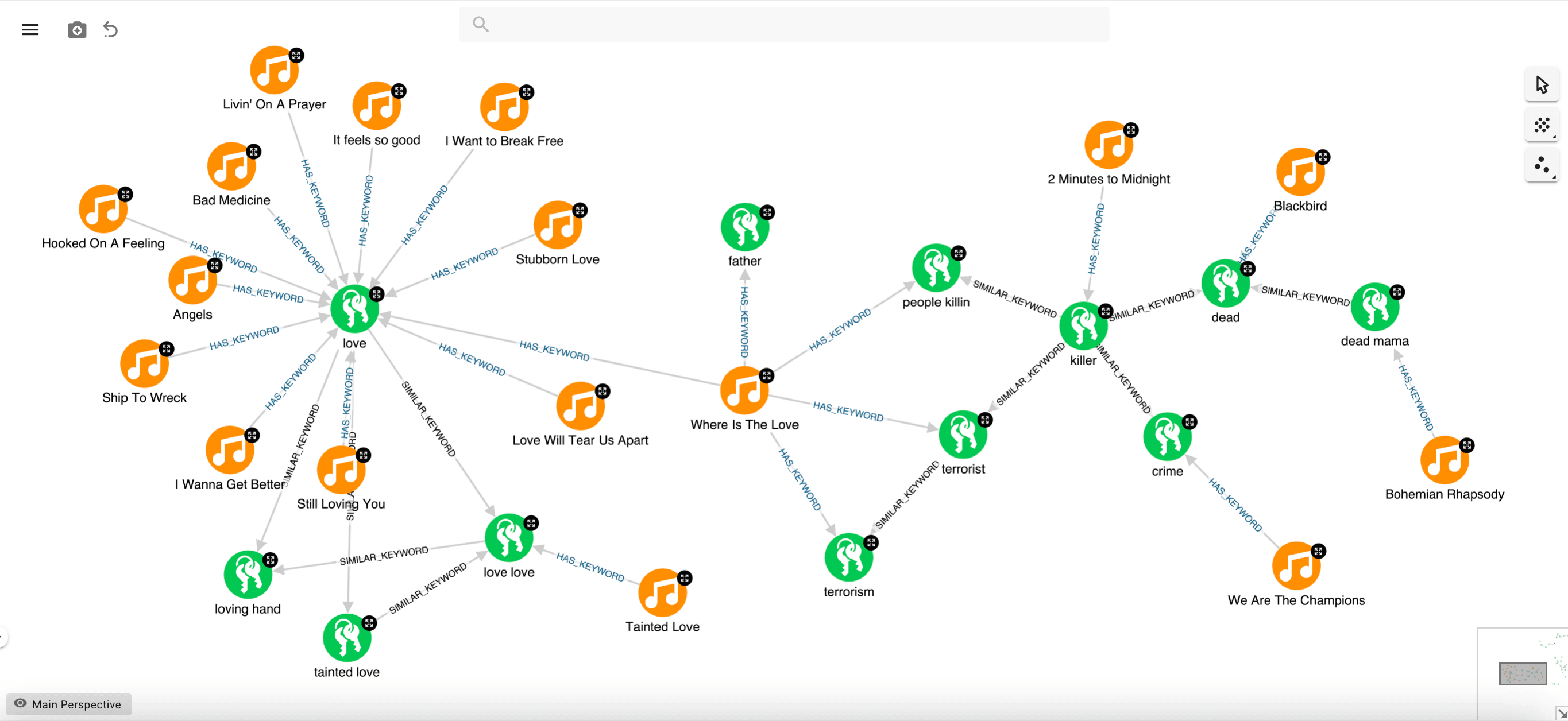
At this point, we came up with another inspiration. Reasoning on the previous example, we realised that it might be useful to consider the whole set of keywords in a song, not just a single keyword, trying to catch its overall message (topic). In this way, we might realise that “Where is The Love” is not really a love song because it clearly has more keywords related to “terrorism” and “killing” than “love.” Based on what we see for this song, we could group the keywords. Example using a community detection algorithm such as strongly connected components, based on the SIMILAR_KEYWORD relationship, so that we can “merge” multiple semantically equivalent expressions (“terrorist”, “terrorism”, “killer”, …) into a single unique entity (keyword cluster). This would make it possible to calculate how closely a song is related to a particular cluster based on the number of keywords that are in that cluster. This way, we could easily find out that “Where is The Love” is much more about killings than love. It is a shame that we could only recover the lyrics of a few songs!

Conclusion

This Song Challenge was really challenging since we started with very limited information. However, we managed to enrich the graph from multiple different sources, set up a recommendation system, find a similarity measure to cluster people based on their musical tastes. Louvain community detection algorithm made this possible and carried out several other analyses, including the final one on the lyrics with keyword extraction and state-of-the-art language model for clustering similar keywords. In other words, it was a complex task, but thanks to Hume ecosystem, we could build it from scratch without any coding effort and have a lot of fun along the way.

To find out more, check out the Neo4j meetup where Luanne and Christophe demonstrated this live: Neo4j Live: A Music Knowledge Graph with GraphAware