- Product
- Industries
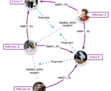
- Law enforcement
Leverage intelligence-led policing with mission-critical graph analytics capabilities.
- Financial authorities
Gain capabilities to act quickly, stop fraud and protect your clients and your business.
- National security
Enable automation, learn about bad actors and their networks, and leverage predictive strategies.
- Law enforcement
- Case studies
- Resources
- Webinars
New use cases, features, and live demos designed to make analysts’ lives easier.
- Books & papers
Our research, philosophy and case studies, all wrapped up in books and papers.
- Videos
Discover GraphAware Hume’s features, demos, and graph technology insights.
- Events
Meet our team at conferences and events around the world.
- Documentation
Review our in-depth user guides and technical documentation to ensure flawless operations.
- Webinars
- Blog
- Company