You’ve seen it in practically every detective series. A map on a wall, covered in pins. Crime scenes, sightings, key locations. Photos and notes pulled into place, each connected by a red string. It’s the moment scattered evidence starts to make sense. Clues become a network, and that network suddenly has a geography.
Outside of TV dramas, investigations rarely work this way. Instead, analysts are working across multiple screens, trying to find connections in data that still lives in silos. Phone records, intelligence reports, suspect histories, location data. Each one living in a different system, accessed through a different tool, analysed in isolation from the rest.
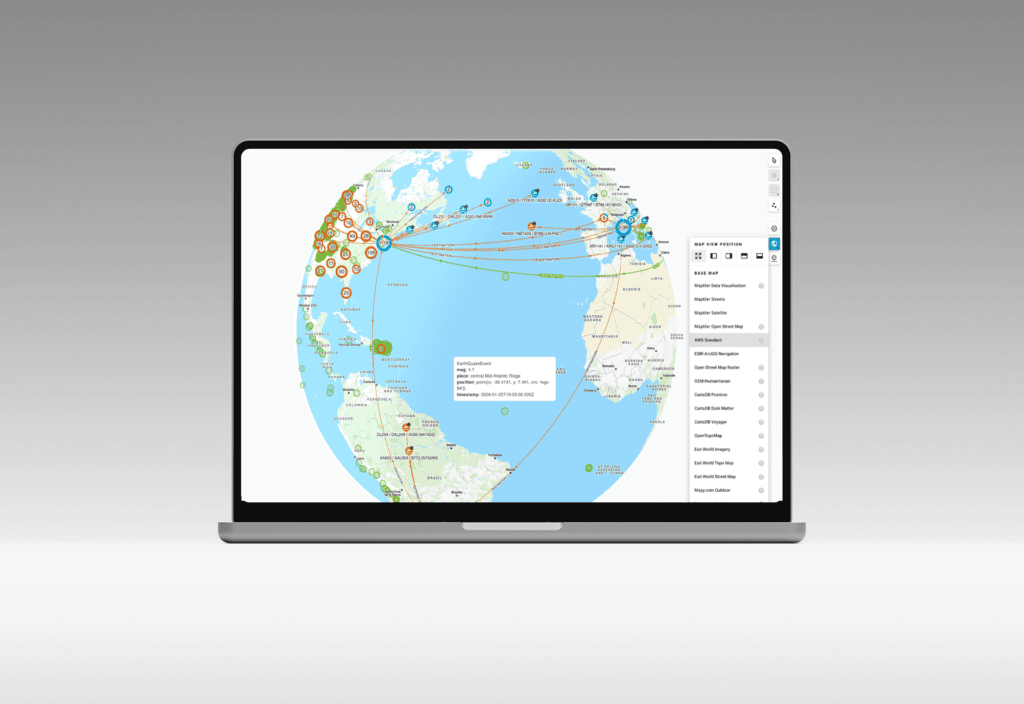
The data is there, so are the connections and the geography. What’s missing is a way to see them together. That’s what geospatial graph analysis does. It combines location and network relationships in a single analytical view, so analysts can see where events occur and how they connect.
This article explains what that means in practice, why it matters, and what it looks like in GraphAware Hume.
Why most teams only ever see part of the picture
Location data sits at the centre of many serious investigations. Phones connect to cell towers. Vehicles travel routes. Transactions occur at locations. Time and place are often the only threads connecting incidents that look, on the surface, unrelated.
But in many intelligence environments, location data is treated as its own separate concern. It lives in different systems from the rest of the investigation. It requires different technology to visualise. Connecting it to the wider picture depends on manual effort, multiple tools, and fragmented workflows.
That separation has real consequences. Analysts spend too much time on tasks that aren’t analysis, such as switching between tools, reformatting data, and manually cross-referencing results. Every switch costs context, and every manual step could lead to missing a connection.
There’s a deeper problem, too. When location data and link analysis are kept apart, certain patterns simply can’t be seen. Not because the information isn’t there, but because no single view ever holds enough of it at once.
Map and graph analysis work better together
Graph-powered intelligence analysis allows analysts to understand how entities connect across an investigation. Geography isn’t background information; it’s evidence. Sometimes it’s the geospatial connection that makes everything else clear.
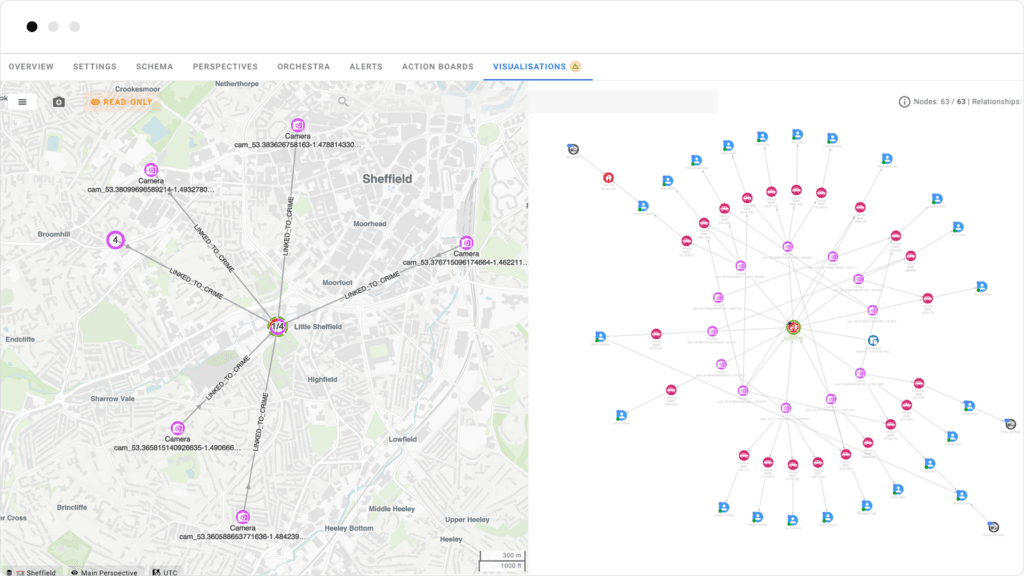
Geospatial graph analysis brings the map view and the graph view together into a unified intelligence picture. The same entities and relationships, anchored in real geography and positioned at their actual coordinates. And crucially, the two views work together. What happens in one is immediately reflected in the other.

The difference this makes becomes clear with an example.
Imagine an analyst is examining a phone dataset with hundreds of contacts and thousands of calls. Looking at the graph view, a pattern stands out. A small number of phones have significantly more connections than the rest, with much higher call volumes. These look like the coordinators.
Then the same data is viewed on the map view.
Those high-activity phones aren’t in the same place. Each one sits at the centre of a cluster of local contacts in a different town or city.
Geographically, what looked like central coordination now looks more like local distribution. And when the full picture is placed in geographic context, something else becomes visible: nearly every regional cluster connects, through only a handful of calls, to a small number of phones concentrated in a single city. Those phones barely stood out in the graph view. But on the map, they’re the point through which every regional cluster connects back to whoever is coordinating from the centre.
The graph view revealed the network structure, and the map view added geographic context, revealing the fuller picture.
Without both views working together, an analyst relying solely on the graph view could have spent significant time focused on the wrong contacts, while the people actually running the operation remained hidden.
What this looks like in GraphAware Hume
As we’ve mentioned, geospatial graph analysis becomes most powerful when applied to real investigations, where connections, location, and time need to be understood together, not in isolation. Here’s what that looks like in practice.
Investigating a series of crimes
A series of incidents occurs across a region, each with a similar method. At first, they appear unrelated. But at one location, CCTV captures a suspicious vehicle, giving analysts a starting point.
Viewed geographically, a clearer sequence of events begins to emerge. The incidents suggest a possible route based on their locations and timing. This guides further analysis. ANPR data along that route is examined, additional sightings are identified, and a set of candidate vehicles starts to take shape.
As more data is added, the graph view and map view reinforce each other. Vehicles stand out not just because of their connections, but because of where and when they appear. From there, analysts can explore how those vehicles link to registered owners or known individuals within the wider intelligence picture. Together, both perspectives allow the analyst to move from a set of disconnected incidents to a coherent, testable picture of what happened.
Digital forensics
A forensic extraction from a suspect’s device gives analysts call logs, contact lists, SMS records, and some location history. On its own, it shows activity within a single device, where numbers and identifiers have limited meaning. When connected to the wider intelligence picture, those identifiers can be resolved to known individuals and linked to existing intelligence, turning isolated data into a more complete, contextualised view of activity.
In GraphAware Hume, that’s exactly what analysts can do. Extraction data sits alongside the wider investigation, so a device’s place in the broader network becomes clear.
Location and time then add context. Analysts can focus on specific periods and explore where a device was likely to be, helping to place individuals near events or identify where multiple devices appear in the same area at similar times. Geospatial, temporal, and graph analysis work as one, without switching tools.
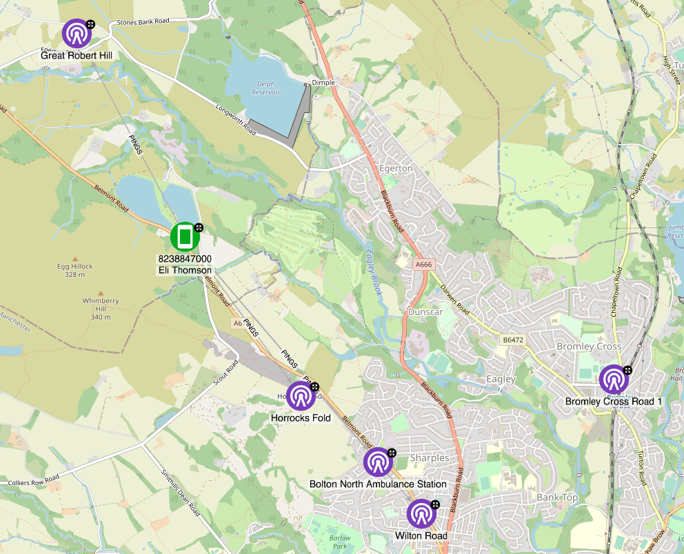
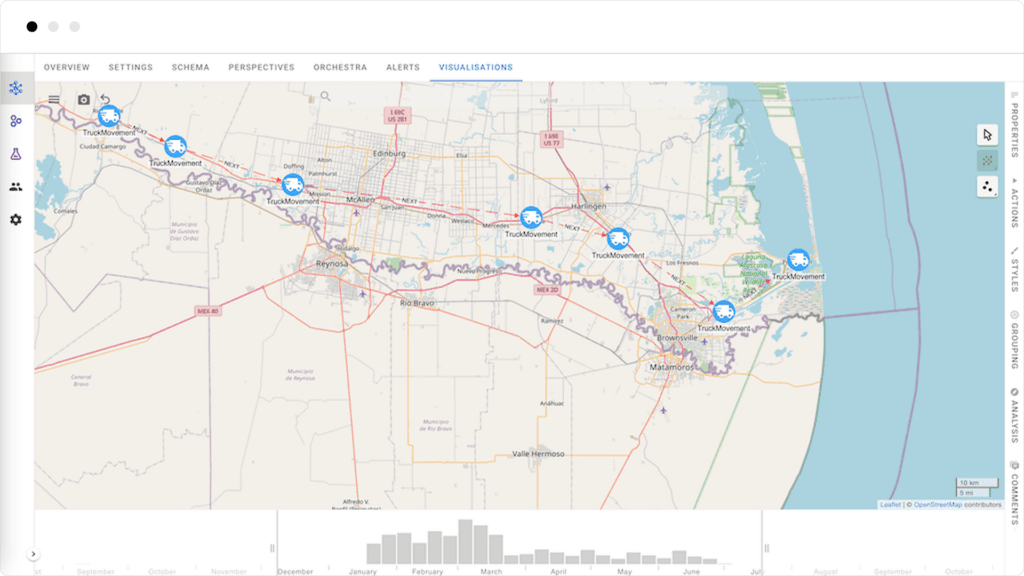
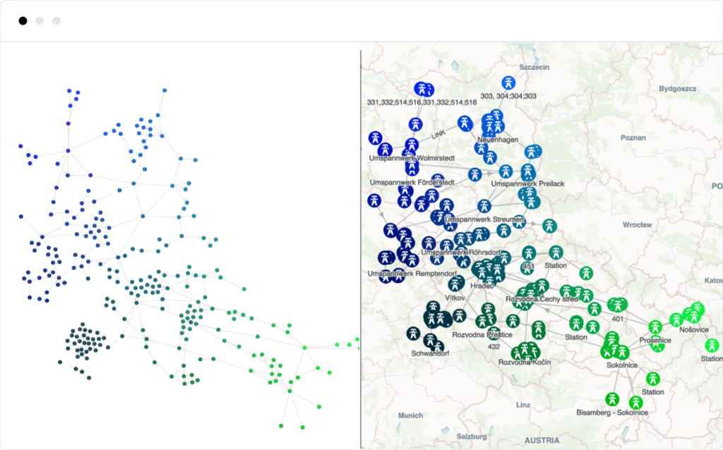
National infrastructure analysis
A team responsible for protecting critical infrastructure, like a power network, needs to understand how exposed it is to hybrid attacks. Knowing where the substations and transmission lines are is only part of the picture. The more important question is how they depend on each other, and which sites, if targeted, would cause the most disruption across the wider network.
In GraphAware Hume, the connected infrastructure can be viewed on a map. The graph view shows how they depend on each other, and the map view shows where they sit. Together, they reveal which sites play the most critical roles in the network’s connectivity, where single points of failure sit, and how a disruption at one location might cascade through the rest. That’s the foundation for knowing where protection matters most.
What geospatial graph analysis requires to work properly
Not every implementation of geospatial graph analysis delivers what analysts actually need. These are the capabilities that matter.
A truly unified view: The map and graph views need to work on the same connected intelligence picture, with changes in one view reflected immediately in the other. A split view that lets analysts see both simultaneously, with selections and expansions mirrored across both, is fundamental to making the method work in practice.
Handling density: In a graph, node position is flexible and can be arranged to reveal structure. On a map, position is fixed by geography, which means dense areas can quickly become cluttered and harder to interpret. Tools need to handle this through proximity clustering: grouping nearby entities at a given zoom level, and expanding or collapsing cleanly when the analyst zooms in or out. The direction of connections should remain clear throughout.
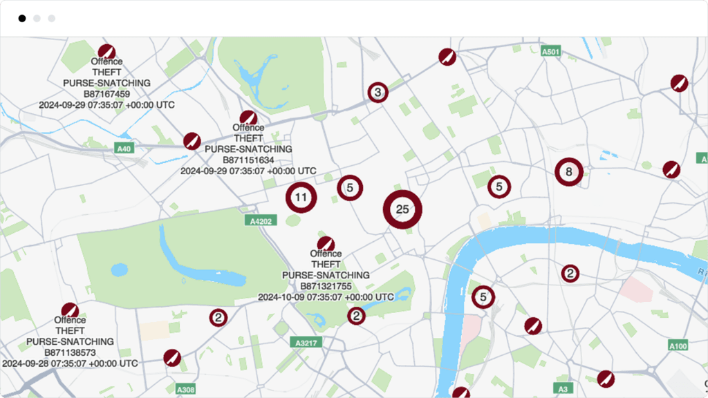
Communicating findings clearly: Maps are an intuitive way to communicate findings to supervisors, other teams, and decision-makers, but only if the view remains clear. Cluttered labels and overlapping connections quickly undermine understanding. Labels and annotations should adjust automatically so the view stays readable and shareable without manual cleanup.
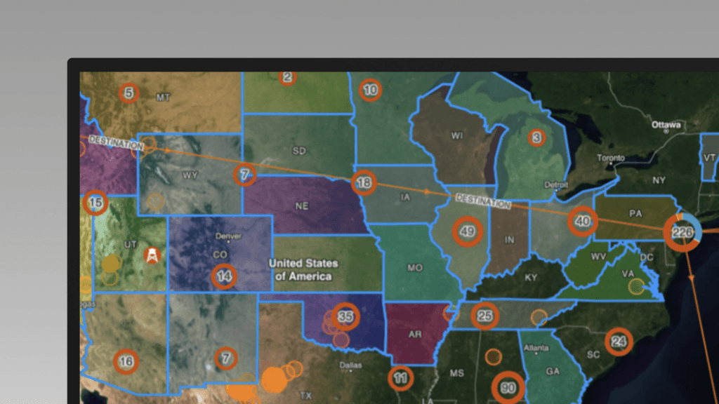
The choice of base map matters too. Different tasks call for different geographic context. Satellite imagery works well for physical surveillance or infrastructure analysis. Street maps help place activity in an urban context. Simplified boundary views can make it easier to communicate findings across a wider area. Tools should support multiple map styles that analysts can switch between depending on what the data needs.
Custom data layers: Analysts need to bring their own geographic data into the same view as the investigation: operational boundaries, infrastructure maps, and probability areas built from signal data. These should sit on the same canvas as the investigation data and be available for analysis alongside it.
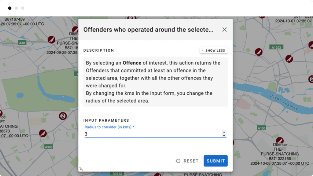
Location-aware actions: The map should work as a direct interface to the data. An analyst should be able to select an area and immediately retrieve what’s relevant nearby, without leaving the view or entering coordinates manually.
Secure deployment: Many organisations working in this space operate in restricted environments where external services are unavailable or not permitted. Tools need to support flexible deployment options, including private and air-gapped environments, without relying on external mapping services.
Stop translating between tools, start seeing the full picture
Location and connections are inseparable in serious investigations. The where and the how are rarely independent questions. But when the tools used to answer them are kept separate, each one gives only part of the picture, and the missing piece is often the one that matters most.
Geospatial graph analysis, done properly, closes that gap. It’s not a map feature or a graph feature. It’s a method that makes both more powerful by combining them, surfacing patterns that stay hidden when location and link analysis operate in isolation.
GraphAware Hume already delivers the core of that method. The map view and graph view share the same connected intelligence foundation, designed to reveal more as complexity grows. And we’re building on it. Richer geometry support, tighter map-graph interaction, and more scalable layer handling are all areas we’re actively exploring. Because the harder the investigation, the more it depends on both views working together.